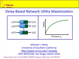
Michael J Neely University of Southern California httpwwwrcfuscedumjneely IEEE INFOCOM San Diego March 2010 Sponsored in part by the DARPA ITMANET Program NSF Career CCF 0747525 ID: 661661
Download Presentation The PPT/PDF document "Delay-Based Network Utility Maximization" is the property of its rightful owner. Permission is granted to download and print the materials on this web site for personal, non-commercial use only, and to display it on your personal computer provided you do not modify the materials and that you retain all copyright notices contained in the materials. By downloading content from our website, you accept the terms of this agreement.
Slide1
Delay-Based Network Utility Maximization
Michael J. NeelyUniversity of Southern Californiahttp://www-rcf.usc.edu/~mjneelyIEEE INFOCOM, San Diego, March 2010
*Sponsored in part by the DARPA IT-MANET Program,
NSF
Career CCF-0747525
a
1
(t)
a
2
(t)
a
K
(
t
)
Utility
Thruput
x
k
S
1
(t)
S
2
(
t)
S
K
(
t
)Slide2
Network Model: 1-Hop Network with K
Queues --- (Q1(t), …, QK(t))Slotted time, t in {0, 1, 2, … }
S(t) = (S1(t), …, SK
(t)) = “Channel State Vector”
(i.i.d. over slots)x(t) = (x1(t), …, x
K(t)) = “Transmission Decision Vector”
a(t) = (a1(t), …, aK(
t)) = “Packet Arrival Vector” (i.i.d. over slots
)Fixed Length Packets: a(t), x(t) are 0/1 vectors.
Arrival Rates: E{a(t)} = (λ1, …, λ
K). Reliability is a Function of Transmission Decision:
Observe S(t) every slot. Choose 0/1 transmission vector x(t).
Pr[Success on link k | x(t
), S(t)] = Ψk(x(t), S(t
))
a
k
(t)
Ψ
k(x(t
), S(t))Slide3
Packet Dropping
:
We can decide to
drop packets at any time.
Packets that fail in transmission can either be retransmitted or dropped.Thruput on channel k = yk = λk – drop rate on channel
k
a
k
(t)
Ψk
(x(t), S(t))
Delay-Based Control
: Stamp Head-of-Line (HOL) Packets with their Delays H
k(t).
Utility Maximization Objective: Maximize: g1( y1 ) + g2
( y2 ) + … + gK( yK
)
where gk(y) are concave, non-decreasing utility functions
Delay
= 4
Delay
= 2
Delay
= 1
Dropsk(t)
Queue k
: Hk(t) = 4 Slide4
Prior work on Stochastic Network Optimization:
Stability: (“Max-Weight” = “Min-Lyapunov-Drift”)
Tassiulas, Ephremides [1992, 1993] (Minimize drift
Δ(t
))Kahale, Wright [1997]Andrews et. al. [2001]Neely, Modiano, Rohrs [2003, 2005]Kobayashi,
Caire, Gesbert [2005]
Joint Stability and Utility Optimization:Neely, Modiano [2003, 2005]
(Minimize Δ(t
) + V*Penalty(t))Georgiadis, Neely, Tassiulas
[2006]Stolyar [2005] (Primal-Dual “Fluid Model” analysis)
Special case of “Infinitely Backlogged Sources”: Agrawal, Subramanian [2002], Kushner, Whiting [2002]
Eryilmaz, Srikant [2005], Lin, Shroff [2004]
All of these references use queue backlog
as weights!Slide5
Alternative “Delay-Based” Rules that use HOL Delaysas weights are known only for
Network Stability:Mekkittikul, McKeown [1996]
Shakkottai, Stolyar [2002]Andrews, Kumaran
, Ramanan, Stolyar
, Vijaykumar, Whiting [2004]Our work fills the gap by developing a Delay-BasedRule for
Maximizing Network Utility Subject to Stability.
a
k
(t)
Ψ
k(x(t), S(t))
Delay
= 4
Delay= 2
Delay
= 1
Drops
k(t)
Utility
Thruput
xkSlide6
Challenges:
Prior “Drift-Plus-Penalty” Algorithm Admit/Drops Packets Immediately when New Packets Arrive: Δ(t) + V*Penalty(t).This does not directly Affect the HOL Values!Tricky Correlation Issues between HOL sizes and Decisions!
Key Ideas for this paper:
Queue all packets. Admit/Drop only at HOL.Use “Drift-Plus-Penalty” with a different queue structure
Use a “concavely extended utility function”Advantages of Delay-Based Approach:Provides “Delay-Fairness.” Queue-Based Rules canleave loner packets stranded.Provides Worst Case Delay Guarantees.
Disadvantage: Must know (λ1, …, λ
K) to implement.Slide7
Concavely Extending a Utility Function:
0
1
y
k
g
k
(y
k)
0
1
y
k
f
k
(y
k
)
-1
slope =
η
k
s
lope
=
η
k
Function
g
k
(y
k):Defined over 0 ≤ yk ≤ 1
Function fk(yk):Defined over -1 ≤ yk ≤ 1 Slide8
Transformed Stochastic Net Optimization Problem:
Maximize: f1( θ
1 ) + f2( θ2
) + … + fK
( θK )Subject to: (1) E{Qk} < infinity , for all k in {1, …, K} (2)
yk ≥ θk , for all
k in {1, …, K} (3) -1 ≤ θk
(t) ≤ 1 , for all t (4) y
k, θk are time averages achievable on the network
Auxiliary Variables and Thruput
Variables:
yk(t) = λk – Drops
k(t) Time Avg:
yk = λk – D
k θ
k(t), choose s.t. -1 ≤ θk(t
) ≤ 1 Time Avg: θk
Slide9
Transformed Stochastic Net Optimization Problem:
Maximize: f1( θ
1 ) + f2( θ2
) + … + fK
( θK )Subject to: (1) E{Qk} < infinity , for all k in {1, …, K} (2)
yk ≥ θk , for all
k in {1, …, K} (3) -1 ≤ θk
(t) ≤ 1 , for all t (4) y
k, θk are time averages achievable on the network
Auxiliary Variables and Thruput
Variables:
yk(t) = λk – Drops
k(t) Time Avg:
yk = λk – D
k θ
k(t), choose s.t. -1 ≤ θk(t
) ≤ 1 Time Avg: θk
Slide10
Transformed Stochastic Net Optimization Problem:
Maximize: f1( θ
1 ) + f2( θ2
) + … + fK
( θK )Subject to: (1) E{Qk} < infinity , for all k in {1, …, K} (2)
yk ≥ θk , for all
k in {1, …, K} (3) -1 ≤ θk
(t) ≤ 1 , for all t (4) y
k, θk are time averages achievable on the network
Virtual Queue Z
k(t) for enforcing constraint (2):
Z
k
(t
)
y
k
(t
) =
λ
k
–
Drops
k
(t)
θk(t)Slide11
Head-of-Line Delay Update Equation (Queue
k):Hk(t+1) = 1{k
full}(t) max[Hk(t
) + 1 – (μk(t)+Dk
(t))Tk(t), 0] + 1{k empty}(t) Ak(t)
Inter-Arrival Time
Tk
(t)
Drops
Service
Lyapunov
Function:
L(t
) = (1/2)[H1(t)2 + … + HK(t)
2] + (1/2)[Z1(t)2 + … + ZK(t)
2] Drift-Plus-Penalty Approach:
Observe {H1(t), …, HK(t)}, {Z
1(t),…,ZK(t)}, {S1
(t), …, SK(t)}Take action to minimize:
Δ
(t) – V [f1(
θ1(t
)) + ... + fK(
θK(t))] Slide12
Resulting Algorithm:
(Aux Variables) Each
k observes Zk(t
). Choose θ
k(t) to: Maximize : V f(θk(t
)) – Zk(t)θk
(t) Subject to: -1 ≤ θk(t
) ≤ 12) (Transmission) Observe S(t), H(t
), Z(t). Choose x(t) to:
Maximize : x
k(t) min[Hk(t), Z
k(t)] Ψk(x(t),S(t))
Subject to: (x1(t),…, xK
(t)) a 0/1 vector3) (Packet Dropping) For each queue k
with HOL packet that was not successfully transmitted, drop iff Z
k(t)≤Hk(t).4) (Update Virtual and Actual Queues)
Δ
(t) – V [f1
(θ1(
t)) + ... + fL
(θL(t
))] ΣkSlide13
Focus on Auxiliary Variable Update:
Choose θk(t)
to: Maximize : V f(θk
(t)) – Zk
(t)θk(t) Subject to: -1 ≤ θk(t) ≤ 1
Key Lemma: If
Zk(t) > Vη
k, then… …the above chooses
θk(t) = -1
…hence, Zk
(t) cannot increase on that slot:
Z
k(t)
y
k
(t) = λ
k – Dropsk(t)
θk(t)
= -1
≥ -1
[This is why we concavely extended the utility function over -1 ≤
y
≤ 1 ]
-1
1
Z
k
(t
)
<
V
η
kSlide14
Focus on Auxiliary Variable Update:
Choose θk(t)
to: Maximize : V f(θk
(t)) – Zk
(t)θk(t) Subject to: -1 ≤ θk(t) ≤ 1
Key Lemma: If
Zk(t) > Vη
k, then… …the above chooses
θk(t) = -1
…hence, Zk
(t) cannot increase on that slot:
Z
k(t)
y
k
(t) = λ
k – Dropsk(t)
θk(t)
= -1
≥ -1
[This is why we concavely extended the utility function over -1 ≤
y
≤ 1 ]
-1
1
Z
k
(t
)
>
V
η
kSlide15
Concluding Theorem:
Implementing the above algorithm for any parameterV>0, we have… Delay: Worst Case Delay in Queue k ≤ Vηk + 2 slots.
Total Utility Satisfies:
g1( y1
) + … + gK( yK ) ≥ g1( y1*)
+ … + gK( yK
*) – B/V
Achieved Utility
Optimal Utility
V
V
Utility
DelaySlide16
Concluding Theorem:
Implementing the above algorithm for any parameterV>0, we have… Delay: Worst Case Delay in Queue k ≤ Vηk + 2 slots.
Total Utility Satisfies:
g1( y1
) + … + gK( yK ) ≥ g1( y1*)
+ … + gK( yK
*) – B/V
Achieved Utility
Optimal Utility
V
V
Utility
DelaySlide17
Concluding Theorem:
Implementing the above algorithm for any parameterV>0, we have… Delay: Worst Case Delay in Queue k ≤ Vηk + 2 slots.
Total Utility Satisfies:
g1( y1
) + … + gK( yK ) ≥ g1( y1*)
+ … + gK( yK
*) – B/V
Achieved Utility
Optimal Utility
V
V
Utility
DelaySlide18
Concluding Theorem:
Implementing the above algorithm for any parameterV>0, we have… Delay: Worst Case Delay in Queue k ≤ Vηk + 2 slots.
Total Utility Satisfies:
g1( y1
) + … + gK( yK ) ≥ g1( y1*)
+ … + gK( yK
*) – B/V
Achieved Utility
Optimal Utility
V
V
Utility
DelaySlide19
Concluding Theorem:
Implementing the above algorithm for any parameterV>0, we have… Delay: Worst Case Delay in Queue k ≤ Vηk + 2 slots.
Total Utility Satisfies:
g1( y1
) + … + gK( yK ) ≥ g1( y1*)
+ … + gK( yK
*) – B/V
Achieved Utility
Optimal Utility
V
V
Utility
DelaySlide20
Concluding Theorem:
Implementing the above algorithm for any parameterV>0, we have… Delay: Worst Case Delay in Queue k ≤ Vηk + 2 slots.
Total Utility Satisfies:
g1( y1
) + … + gK( yK ) ≥ g1( y1*)
+ … + gK( yK
*) – B/V
Achieved Utility
Optimal Utility
V
V
Utility
DelaySlide21
Concluding Theorem:
Implementing the above algorithm for any parameterV>0, we have… Delay: Worst Case Delay in Queue k ≤ Vηk + 2 slots.
Total Utility Satisfies:
g1( y1
) + … + gK( yK ) ≥ g1( y1*)
+ … + gK( yK
*) – B/V
Achieved Utility
Optimal Utility
V
V
Utility
DelaySlide22
Concluding Theorem:
Implementing the above algorithm for any parameterV>0, we have… Delay: Worst Case Delay in Queue k ≤ Vηk + 2 slots.
Total Utility Satisfies:
g1( y1
) + … + gK( yK ) ≥ g1( y1*)
+ … + gK( yK
*) – B/V
Achieved Utility
Optimal Utility
V
V
Utility
DelaySlide23
Example Utility Function
gk( y ) = log( 1 + ηk
y )This approximates “proportionally fair” log-utility
when η
k is large. The log-utility log( y ) has a singularity at y=0, and so
is not always a good choice of utility function.
V
V
Utility
Delay