
Chapter 5 DiscreteTime Process Models DiscreteTime Transfer Functions The input to the continuoustime system G s is the signal The system response is given by the convolution integral ID: 814646
Download The PPT/PDF document "Now let us calculate the transient respo..." is the property of its rightful owner. Permission is granted to download and print the materials on this web site for personal, non-commercial use only, and to display it on your personal computer provided you do not modify the materials and that you retain all copyright notices contained in the materials. By downloading content from our website, you accept the terms of this agreement.


Slide1
Slide2Now let us calculate the transient response of a combined discrete-time and continuous-time system, as shown below.
Chapter 5
Discrete-Time Process Models
Discrete-Time Transfer Functions
The input to the continuous-time system
G(s) is the signal:
The system response is given by the convolution integral:
Slide3With
Chapter 5
Discrete-Time Process Models
Discrete-Time Transfer Functions
For 0 ≤
τ
≤
t,
We assume that the output sampler is ideally synchronized with the input sampler.
The output sampler gives the signal
y
*
(
t
) whose values are the same as
y
(
t
) in every sampling instant
t
= jTs.
Applying the
Z
-transform yields:
Slide4Chapter 5
Discrete-Time Process ModelsDiscrete-Time Transfer Functions
Taking
i
= j – k
, then:
For zero initial conditions,
g(iT
s) = 0, i < 0, thus:
where
Discrete-time Transfer Function
The
Z
-transform
of Continuous-time Transfer Function
g
(
t
)
The
Z
-transform
of
Input Signal
u
(
t
)
Slide5Chapter 5
Discrete-Time Process ModelsDiscrete-Time Transfer Functions
Y
(
z
) only indicates information about y(t) in sampling times, since G(z
) does not relate input and output signals at times between sampling times.
When the sample-and-hold device is assumed to be a zero-order hold, then the relation between G(s) and G(z) is
Slide6Chapter 5
Discrete-Time Process ModelsExample
Find the discrete-time transfer function of a continuous system given by:
where
Slide7Chapter 5
Discrete-Time Process ModelsInput-Output Discrete-Time Models
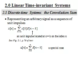
A general discrete-time linear model can be written in time domain as:
where
m
and
n
are the order of numerator and denominator, k denotes the time instant, and d is the time delay.
Defining a shift operator
q–1, where:
Then, the first equation can be rewritten as:
or
Slide8Chapter 5
Discrete-Time Process ModelsInput-Output Discrete-Time Models
The polynomials
A
(q–1) and
B(q–1) are in descending order of q–1, completely written as follows:
The last equation on the previous page can also be written as:
Hence, we can define a function:
Identical, with the difference only in the use of notation for shift operator,
q
-1
or
z
–1
Slide9Chapter 5
Discrete-Time Process ModelsApproximation of
Z-Transform
Previous example shows how the
Z-transform of a function written in s
-Domain can be so complicated and tedious.Now, several methods that can be used to approximate the Z-transform will be presented.
Consider the integrator block as shown below:
The integration result for one sampling period of
T
s
is:
Slide10Chapter 5
Discrete-Time Process Models
Forward Difference Approximation
(Euler Approximation)
The exact integration operation presented before will now be approximated using Forward Difference Approximation.
This method follows the equation given as:Approximation of Z-Transform
Taking the
Z
-transform
of the above equation:
while
Thus, the Forward Difference Approximation is done by taking
or
Slide11Chapter 5
Discrete-Time Process Models
Backward Difference Approximation
The exact integration operation will now be approximated using Backward Difference Approximation.
This method follows the equation given as:
Approximation of Z-Transform
Taking the
Z
-transform
of the above equation:
while
Thus, the
Backward Difference
Approximation is done by taking
or
Slide12Chapter 5
Discrete-Time Process Models
Trapezoidal Approximation
(Tustin Approximation, Bilinear Approximation)
The exact integration operation will now be approximated using Backward Difference Approximation.
This method follows the equation given as:
Taking the
Z
-transform
,
while
Thus, the
Trapezoidal Approximation
is done by taking
or
Approximation of
Z
-Transform
Slide13Chapter 5
Discrete-Time Process ModelsExample
Find the discrete-time transfer function of
for the sampling time of
T
s = 0.5 s, by using (a) ZOH, (b) FDA, (c) BDA, (d) TA.
(a) ZOH
(b) FDA
Slide14Chapter 5
Discrete-Time Process ModelsExample
(c) BDA
(d) TA
Slide15Chapter 5
Discrete-Time Process ModelsExample
ZOH
FDA
TA
BDA
Slide16Chapter 5
Discrete-Time Process ModelsExample: Discretization of Single-Tank System
Retrieve the
linearized model
of the single-tank system. Discretize the model using trapezoidal approximation, with
Ts = 10 s.
Laplace Domain
Z
-Domain
Slide17Chapter 5
Discrete-Time Process ModelsExample: Discretization of Single-Tank System
Slide18Chapter 5
Discrete-Time Process ModelsExample: Discretization of Single-Tank System
Slide19Chapter 5
Discrete-Time Process ModelsExample: Discretization of Single-Tank System
:
Linearized
model
:
Discretized l
inearized model
Slide20Chapter 5
Discrete-Time Process ModelsExample: Discretization of Single-Tank System
:
Linearized
model
:
Discretized l
inearized model
Slide21Chapter 5
Discrete-Time Process ModelsHomework 8
(a) Find
the discrete-time transfer functions of the following continuous-time transfer function, for
Ts = 0.25 s and
Ts = 1 s. Use the Forward Difference Approximation
(b) Calculate
the step response of both
discrete transfer functions for
0 ≤ t ≤ 5 s.(c) Compare the step response of both transfer functions with the step response of the continuous-time transfer function G(s
) in one plot/scope for 0 ≤
t
≤ 0.5 s.
Slide22Chapter 5
Discrete-Time Process ModelsHomework 8A
Find
the discrete-time transfer functions of the following continuous-time transfer function, for
Ts = 0.1 s and
Ts = 0.05 s. Use the following approximation:Forward Difference
(Andre, Burawi, Deom, Indah, Jagat)
Backward Difference (Arief, Arwin, Keanu, Yeza, Wilbert)
(b) Calculate
the step response of both
discrete transfer
functions for
0
≤
t
≤ 0.5
s. The calculation for
t
=
kT
s, k = 0 until k
= 5 in each case must be done manually. The rest may be done by the help of Matlab Simulink.(c) Compare the step response of both discrete transfer functions with the step response of the continuous-time transfer function
G(s) in one plot/scope for 0 ≤ t ≤ 0.5 s.
Deadline: Thursday,
21 March 2019
.