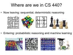
Where are we in CS 440? Now leaving: sequential, - PowerPoint Presentation

Slide1

Where are we in CS 440?

Now leaving: sequential, deterministic reasoningEntering: probabilistic reasoning and machine learning

Slide2

Probability: Review of main concepts (Chapter 13)

Slide3

Making decisions under uncertainty

Let action

A

t

= leave for

airport

t

minutes

before flight

Will

A

t

succeed, i.e., get

me

to the airport in time for the flight?

Problems

:

Partial

observability

(road state, other drivers' plans, etc

.)

Noisy

sensors (traffic reports

)

Uncertainty

in action outcomes (flat tire, etc

.)

Complexity

of modeling and predicting

traffic

Hence a

non-probabilistic approach

either

Risks

falsehood: “

A

25

will get me there on

time,”

or

Leads

to conclusions that are too weak for decision making

:

A

25

will get me there on time if there's no accident on the bridge and it doesn't rain and my tires remain

intact, etc.,

etc

.

A

1440

will

get me there on time but

I’ll

have to stay overnight in the

airport

Slide4

Making decisions under uncertainty

Suppose

the agent believes

the following

:

P(A

25

gets me there on

time) =

0.04

P(A

90

gets me there on

time) =

0.70

P(A

120

gets me there on

time) =

0.95

P(A

1440

gets me there on

time) =

0.9999

Which action

should the agent choose?

Depends

on

preferences

for missing flight vs. time spent

waiting

Encapsulated by a

utility function

The agent should choose the action that maximizes the

expected utility

:

P(A

t

succeeds) * U(A

t

succeeds) + P(A

t

fails) * U(A

t

fails)

Slide5

Making decisions under uncertainty

More generally: the expected utility of an action is defined as:

EU(a) =

Σ

outcomes

of a

P(outcome

|

a) U(outcome)

Utility

theory

is used to represent and infer

preferences

Decision theory

= probability theory + utility

theory

Slide6

Monty Hall problem

You’re a contestant on a game show. You see three closed doors, and behind one of them is a prize. You choose one door, and the host opens one of the other doors and reveals that there is no prize behind it. Then he offers you a chance to switch to the remaining door. Should you take it?

http://en.wikipedia.org/wiki/Monty_Hall_problem

Slide7

Monty Hall problem

With probability 1/3, you picked the correct door, and with probability 2/3, picked the wrong door. If you picked the correct door and then you switch, you lose. If you picked the wrong door and then you switch, you win the prize.

Expected utility of switching:

EU(Switch) = (1/3) * 0 + (2/3) * Prize

Expected utility of not switching:

EU(Not switch) = (1/3) * Prize + (2/3) * 0

Slide8

Where do probabilities come from?

Frequentism

Probabilities are relative frequencies

For example, if we toss a coin many times,

P(heads)

is the proportion of the time the coin will come up heads

But what if we’re dealing with events that only happen once?

E.g., what is the probability that Team X will win the

Superbowl

this year?

“Reference class” problem

Subjectivism

Probabilities are degrees of belief

But then, how do we assign belief values to statements?

W

hat would constrain agents to hold consistent beliefs?

Slide9

Probabilities and rationality

Why should a rational agent hold beliefs that are consistent with axioms of probability?

For example,

P(A) + P(

¬

A) = 1

If an agent has some degree of belief in proposition

A

,

he/she should be able to decide whether or not to accept

a bet for/against

A

(

De

Finetti

, 1931):

I

f the agent believes that

P(

A

) = 0.4

, should he/she agree to bet

$4

that A will occur against

$6

that

A

will not occur?

Theorem:

An agent who holds beliefs inconsistent with axioms of probability can be convinced to accept a combination of bets that is guaranteed to lose them money

Slide10

Random variables

We describe the (uncertain) state of the world using

random variables

Denoted by capital letters

R

:

Is it raining?

W

:

What’s the weather?

D

:

What is the outcome of rolling two dice?

S

:

What is the speed of my car (in MPH)?

Just like variables in CSPs, random variables take on values in a

domain

Domain values must be

mutually exclusive

and

exhaustive

R

in

{True, False}

W

in

{Sunny, Cloudy, Rainy, Snow}

D

in

{(1,1), (1,2), … (6,6)}

S

in

[0,

200]

Slide11

Events

Probabilistic statements are defined over

events

, or sets of world states

“It is raining”

“The weather is either cloudy or snowy”

“The sum of the two dice rolls is 11”

“My car is going between 30 and 50 miles per hour”

Events are described using propositions about random variables:

R = True

W = “Cloudy”

 W = “Snowy”

D

 {(5,6), (6,5)}

30  S  50

Notation:

P(

A

)

is the probability of the set of world states in which proposition

A

holds

Slide12

Kolmogorov’s axioms of probability

For any

propositions (events)

A

,

B

0

≤

P(

A

)

≤

1

P(True

) = 1 and

P(False

) = 0

P(

A



B

)

=

P(

A

)

+

P(

B

) – P(

A



B

)

Subtraction accounts for double-counting

Based on these axioms, what is

P(

¬

A

)

?

These axioms are sufficient to completely specify probability theory for

discrete

random variables

For continuous variables, need

density functions

Slide13

Atomic events

Atomic

event:

a

complete specification of the state of the

world, or a complete assignment of domain values to all random variables

Atomic events are mutually exclusive and exhaustive

E.g

., if the world consists of only two Boolean variables

Cavity

and

Toothache

, then there are

four

distinct atomic

events:

Cavity

= false



Toothache =

false

Cavity

= false



Toothache =

true

Cavity

= true



Toothache =

false

Cavity

= true



Toothache =

true

Slide14

Joint probability distributions

A joint distribution is an assignment of probabilities to every possible atomic eventWhy does it follow from the axioms of probability that the probabilities of all possible atomic events must sum to 1?

Atomic event

P

Cavity = false



Toothache = false

0.8

Cavity = false



Toothache = true

0.1

Cavity = true



Toothache = false

0.05

Cavity = true



Toothache = true

0.05

Slide15

Joint probability distributions

A

joint distribution

is an assignment of probabilities to every possible

atomic event

Suppose

we have a joint distribution of

n

random variables with domain sizes

d

What is the size of the probability table?

Impossible to write out completely for all but the smallest distributions

Slide16

Notation

P(X

1

= x

1

, X

2

= x

2

, …,

X

n

=

x

n

)

refers to a single entry

(atomic event) in the joint probability distribution table

Shorthand:

P(x

1

,

x

2

, …,

x

n

)

P(X

1

, X

2

, …,

X

n

)

refers to the entire joint probability distribution table

P(A)

can also refer to the probability of an event

E.g.,

X

1

=

x

1

is an event

Slide17

Marginal probability distributions

From the joint distribution P(X,Y) we can find the marginal distributions P(X) and P(Y)

P(Cavity, Toothache)Cavity = false Toothache = false0.8Cavity = false  Toothache = true0.1Cavity = true  Toothache = false0.05Cavity = true  Toothache = true0.05

P(Cavity)Cavity = false?Cavity = true ?

P(Toothache

)

Toothache = false

?

Toochache

= true

?

Slide18

Marginal probability distributions

From the joint distribution P(X,Y) we can find the marginal distributions P(X) and P(Y)To find P(X = x), sum the probabilities of all atomic events where X = x: This is called marginalization (we are marginalizing out all the variables except X)

Slide19

Conditional probability

Probability of cavity given toothache: P(Cavity = true | Toothache = true)For any two events A and B,

P(A)

P(B)

P(A

 B

)

Slide20

Conditional probability

What is P(Cavity = true | Toothache = false)?0.05 / 0.85 = 0.059What is P(Cavity = false | Toothache = true)?0.1 / 0.15 = 0.667

P(Cavity, Toothache)Cavity = false Toothache = false0.8Cavity = false  Toothache = true0.1Cavity = true  Toothache = false0.05Cavity = true  Toothache = true0.05

P(Cavity)Cavity = false0.9Cavity = true 0.1

P(Toothache

)

Toothache = false

0.85

Toothache = true

0.15

Slide21

Conditional distributions

A conditional distribution is a distribution over the values of one variable given fixed values of other variables

P(Cavity, Toothache)Cavity = false Toothache = false0.8Cavity = false  Toothache = true0.1Cavity = true  Toothache = false0.05Cavity = true  Toothache = true0.05

P(Cavity | Toothache = true)Cavity = false0.667Cavity = true 0.333

P(Cavity|Toothache = false)Cavity = false0.941Cavity = true 0.059

P(Toothache | Cavity = true)Toothache= false0.5Toothache = true 0.5

P(Toothache | Cavity = false

)

Toothache= false

0.889

Toothache = true

0.111

Slide22

Normalization trick

To get the whole conditional distribution P(X | Y = y) at once, select all entries in the joint distribution table matching Y = y and renormalize them to sum to one

P(Cavity, Toothache)Cavity = false Toothache = false0.8Cavity = false  Toothache = true0.1Cavity = true  Toothache = false0.05Cavity = true  Toothache = true0.05

Toothache, Cavity = falseToothache= false0.8Toothache = true 0.1

P(Toothache | Cavity = false)Toothache= false0.889Toothache = true 0.111

Select

Renormalize

Slide23

Normalization trick

To get the whole conditional distribution P(X | Y = y) at once, select all entries in the joint distribution table matching Y = y and renormalize them to sum to oneWhy does it work?

b

y marginalization

Slide24

Product rule

Definition of conditional probability: Sometimes we have the conditional probability and want to obtain the joint:

Slide25

Chain rule

Product rule:Chain rule:

Slide26

Independence

T

wo events A and B are

independent

if and only if

P(A

 B) = P(A, B) = P(A) P(B)

In other words,

P(A | B) = P(A)

and

P(B | A) = P(B)

This is an important simplifying assumption for modeling, e.g.,

Toothache

and

Weather

can be assumed to be independent

Are two

mutually exclusive

events independent?

No, but for mutually exclusive events we have

P(A  B) = P(A) + P(B)

Slide27

Independence

T

wo events A and B are

independent

if and only if

P(A

 B) =

P(A, B) = P

(A) P(B)

In other words,

P(A | B) = P(A)

and

P(B | A) = P(B)

This is an important simplifying assumption for modeling, e.g.,

Toothache

and

Weather

can be assumed to be independent

Conditional independence

: A and B are

conditionally independent

given C

iff

P(A  B | C) = P(A | C) P(B | C)

Equivalently:

P

(A

| B, C

) = P(A | C)

or P(B

|

A,

C) = P

(B

| C)

Slide28

Conditional independence: Example

Toothache

:

boolean

variable indicating whether the patient has a toothache

Cavity

:

boolean

variable indicating whether the patient has a cavity

Catch

:

whether the dentist’s probe catches in the cavity

If the patient has a

cavity, the probability that the probe catches in it doesn't depend on whether

he/she has a toothache

P(

C

atch

|

Toothache

,

Cavity

) =

P(

Catch

|

Cavity

)

Therefore

,

Catch

is conditionally independent of

Toothache

given

Cavity

Likewise,

Toothache

is conditionally independent of

Catch

given

Cavity

P(

Toothache | Catch, Cavity

) = P(

Toothache | Cavity

)

Equivalent statement:

P(

Toothache

, Catch | Cavity

) = P(

Toothache | Cavity

) P(

Catch | Cavity

)

Slide29

Conditional independence: Example

How many numbers do we need to represent the joint probability table

P(

Toothache, Cavity, Catch

)

?

2

3

– 1 = 7 independent entries

Write

out

the

joint distribution using chain rule

:

P(

Toothache, Catch, Cavity

)

= P(

Cavity

) P(

Catch

|

Cavity

)

P(

Toothache | Catch, Cavity

)

=

P(

Cavity

) P(

Catch

|

Cavity

) P(

Toothache

| Cavity

)

How many numbers do we need to represent these distributions?

1 + 2

+

2

= 5 independent

numbers

In most cases, the use of conditional independence reduces the size of the representation of the joint distribution from exponential in

n

to linear in

n

Slide30

The Birthday problem

We have a set of n people. What is the probability that two of them share the same birthday?Easier to calculate the probability that n people do not share the same birthday

Slide31

The Birthday problem

Slide32

The Birthday problem

For 23 people, the probability of sharing a birthday is above 0.5!

http://en.wikipedia.org/wiki/Birthday_problem