/
Details of polymer chain Details of polymer chain

Details of polymer chain - PowerPoint Presentation

karlyn-bohler
karlyn-bohler . @karlyn-bohler
Follow
343 views
Uploaded On 2019-06-20

Details of polymer chain - PPT Presentation

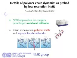
dynamics as probed by lowresolution NMR A Mordvinkin Kay Saalwächter NMR approaches for complex anisotropic rotational diffusion Chain dynamics in polymer melts and ID: 759391

Share:

Link:

Embed:

Download Presentation from below link

Download Presentation The PPT/PDF document "Details of polymer chain" is the property of its rightful owner. Permission is granted to download and print the materials on this web site for personal, non-commercial use only, and to display it on your personal computer provided you do not modify the materials and that you retain all copyright notices contained in the materials. By downloading content from our website, you accept the terms of this agreement.


Presentation Transcript

Slide1

Details of polymer chain

dynamics as probed by low-resolution NMRA. Mordvinkin, Kay Saalwächter

NMR approaches for complex (anisotropic) rotational diffusionChain dynamics in polymer melts and supramolecular networks

Slide2

“Simple NMR”: the potential of integrated 1H signal

Fourier

transformation

HO–CH

2

–CH

3

frequencyspectrum

N

S

spin-1/2

free induction decay

acquisition time

inhom

. low field:

no spectral resolution

couplings, broadening and relaxation...

...encoded in

time-domain

(echo)

decay

Slide3

intermediate

t

c

»

1/Dzz

t

c

(T)

Rotations and averaging of dipolar couplings

static

spectrum

dipolar coupling tensor

D

µ gigj/rij3

Dstat = Dzz » 30 kHz!

fast-limit

spectrum

D

res

µ S (order param.)

q

±

D

(

q

)

B

0

D

zz

D

xx

D

yy

Slide4

Rotational diffusion from relaxation times/rates

isotropic Brownian tumbling removes orientation-dependent interacations from spectra (Dres = 0)but: relaxation times (T1, T2) depend on the timescale of these fast (tr ~ ns) orientation fluctuations

H

H

e.g. dipole-dipole coupling

q

(

t

)

B

0

t

r

described in terms of

orientation autocorrelation functions, e.g. C2,0(t) = <P2[cos q(t)]P2[cos q(t+t)]>t ~ exp{-t/tr}internal motions: Lipari-Szabo (LSz) “model-free” approachC2,0(t) := [(1-S2)exp{-t/tint} + S2]exp{-t/tr}BPP/Redfied theory predicts, e.g., where the spectral density Jr(w) = FT{C(t)} (LSz: just sum of Lorentzians!)

spectral density and

R

i

high-field

R

1

, NOE range

t

r

-1

t

int

-1

log

w

log

J

(

w

)

R

2

(

J

(0))

FT

log-log scale

t

w

S

2

Slide5

Beyond Lipari-Szabo?

log

w

log

J

(

w

)

log

C(t)

log

t

“normal”

Brownian tumbling

correlation function

C

2,0

(

t

) =

C

(

t

)

Þ

spectral density

J

(

w)

power laws?

Slide6

Rouse t <

t

e

(locally unrestricted)

entanglements

or crosslinks

t

e

< t <

t

R

(tube restriction)

reptation

t

R

< t <

t

d

(tube renewal)

Structure and dynamics in polymers: concepts

multi-timescale

dynamics

single-chain (!)

bead-spring

models

l

0

Slide7

Tube model prediction for NMR observable C(t)

see: de Gennes, J. Chem. Phys. 1971!

0

I

II

III

IV

t

1/2

log

<

r

(

t

)

-

r

(0)

2

>

log

t

10

-6

m

t

s

ns

ns –

m

s

m

s – ms

ms – d

ps

t

e

t

R

t

d

10

-8

m

10

-10

m

C

C

C

f

sub-

segmental

free

Rouse

constrained

Rouse

reptation

free

diffusion

t

1/4

t

1/2

t

1

log

C

(

t) ~ S

b

2

1

10

-4

10

-8

t

1

t

1/4

t

1/2

R. C. Ball, P. T. Callaghan,

E. T.

Samulski

,

J. Chem. Phys.

106

(1997) 7352.

Slide8

R. Graf et al.,

Phys. Rev. Lett. 80 (1998) 5783KS, Progr. NMR Spectrosc. 51 (2007) 1-35

spectrum

FID/Hahn echo

dipolar time evolution (coupling changes with time!)

freq.

t

echo

FT

convoluted

signal decay,

ambiguous

analysis

MQ vs

T

2

: more meaningful signal functions!

Transverse relaxation vs. MQ spectroscopy

½

t

echo

½

t

echo

p

I

echo

separated effects:

S

MQ – segmental

dynamics (

a

=

f

(

t

<

t

e

) )

D

Q –

local order

(

D

res

,

b

)

and reptation (

b

=

f

(

t>

t

e

))

MQ experiment

mobile

parts (ends)

t

DQ

t

DQ

t

DQ

DQ

reconversion

DQ

excitation

I

S

MQ

/

DQ

vs.

Slide9

MQ time-domain NMR: networks vs. melts

KS, A. Heuer, Macromolecules 39 (2006) 3291-3303

normalized DQ build-up in networks C(t) plateau due to crosslinks C(t) ~ Sb2 ~ Dres2 ~ 1/Mc2

0.5

S

MQ relaxation:

incoherent

dynamics

DQ

nDQ =

DQ

/

S

MQ

:

local order µ C(tDQ)

example: natural rubber

0

2

4

6

8

10

0.0

0.2

0.4

0.6

0.8

1.0

norm. intensity

DQ evolution time / ms

S

MQ

DQ

nDQ

0

2

4

6

DQ evolution time / ms

vulcanized (3 phr sulfur)

403K

285K

340K

10

-

5

10

-

4

10

-

3

10

-

2

10

-

1

10

0

10

1

10

2

10

3

10

4

10

5

10

6

10

7

10

-

6

10

-

5

10

-

4

10

-

3

10

-

2

10

-

1

10

0

C

(

t

/

t

e

)

t

/

t

e

(

T

)

nDQ

0

2

4

6

DQ evolution time / ms

0

2

4

6

8

10

DQ evolution time / ms

S

MQ

DQ

403K

285K

340K

linear precursor polymer

segmental dynamics!

tube constraint, reptation!

segmental dynamics!

network chain structure (

S

) !

Slide10

Scaling analysis of MQ NMR observable and TTS

0.0

0.2

0.4

0.6

0.8

1.0

1.2

1.4

1.6

1.8

0.0

0.1

0.2

0.3

0.4

0.5

PB2000k (

Z

=1100)

t

2

DQ

C

(

t

)

absolute-value fit

243 K

303 K

363 K

norm. DQ intensity

validity limit

t

DQ

/ ms

TTS

–0.29

TTS

other temperatures

TTS

initial

nDQ signal

10

0

10

1

10

2

10

3

10

4

10

5

10

-6

10

-5

10

-4

10

-3

0.1

1

10

-4

10

-3

C

(

t

/

t

e

)

243 K

303 K

363 K

t

DQ

[ms]

C

(

t

DQ

) ~

I

nDQ

/

t

DQ

2

t

/

t

e

PB2000k (

Z

=1100)

use

time-temperature

superposition

to obtain

C

(

t

/

t

e

,

T

ref

):

see: R. Graf et al.,

Phys. Rev. Lett.

80

(1998) 5783

Slide11

t

-

0.85

I

0

PB2.8k (

Z

=1.5)

PB4.6k (

Z

=3)

PB9.5k (

Z

=5)

PB11.4k (

Z

=8)

PB18k (

Z

=10)

T

1

field

cycling

(Herrmann

et al

.)

A. Herrmann, V. N. Novikov, E. A. Rössler,

Macromolecules

42

(2009) 2063.

field cycling NMR

Full time range by NMR

10

-4

10

-3

10

-2

10

-1

10

0

10

1

10

2

10

3

10

4

10

5

10

-8

10

-7

10

-6

10

-5

10

-4

10

-3

10

-2

10

-1

10

0

10

1

t

/

t

e

C

(

t

/

t

e

)

PB23k (

Z

=12)

PB35k (

Z

=19)

PB87k (

Z

=47)

PB2000k (

Z

=1100)

low-field

MQ NMR

(our

work)

II

III,IV

F. V. Chavez, KS,

Phys. Rev. Lett.

104

(2010) 198305.

Slide12

Analytical treatment and MQ data fitting

KS, A. Heuer,

Macromolecules 39 (2006) 3291-3303F.V. Chavez, KS, Macromolecules 44 (2011) 1560-1569.

use the second-moment (Anderson-Weiss) approximationto calculate signal functions, e.g.

averages

over

phase factors reduce to integrals over C(t), e.g.

time

0

frequency

FT

assumption

:

Gaussian

freq. distribution

Þ

not valid

at

long

times!

½

t

echo

½

t

echo

p

I

echo

t

DQ

t

DQ

2: DQ reconv.

1: DQ exc.

I

S

MQ/DQ

vs.

Slide13

Analytical predictions based upon full (known) C(t)

0

2

4

6

8

10

12

14

16

18

20

0.0

0.2

0.4

0.6

0.8

1.0

273 K

PB 87 kDa

353 K

0

2

4

6

8

10

12

14

16

18

20

0.0

0.2

0.4

0.6

0.8

1.0

normalized intensity

PB 35 kDa

0

2

4

6

8

10

12

14

16

18

20

0.0

0.2

0.4

0.6

0.8

1.0

normalized intensity

t

DQ

[ms]

PB 441 kDa

0

2

4

6

8

10

12

14

16

18

20

0.0

0.2

0.4

0.6

0.8

1.0

PB 2000 kDa

t

DQ

[ms]

S

MQ

DQ

273 K

363 K

343 K

273 K

353 K

273 K

MQ data

F.V. Chavez, KS,

Macromolecules

44

(2011) 1560-1569.

0

2

4

6

8

10

0.0

0.2

0.4

0.6

0.8

1.0

normalized Hahn echo intensity

0

2

4

6

8

10

0.0

0.2

0.4

0.6

0.8

1.0

normalized Hahn echo intensity

t

echo

[ms]

273 K

363 K

PB 2000 kDa

PB 35 kDa

273 K

343 K

Hahn echo

data

no

free

parameters

!

clearly

non-

exponential

!

Slide14

just an

exponential

T2 term for dynamics at t < t0=tDQmin!

Minimal fitting model

A.

Mordvinkin, KS, J. Chem. Phys. 146 (2017) 094902;Erratum: 148 (2018) 089901

*KS, A. Heuer,

Macromolecules 39 (2006) 3291-3303

analytical result (AW approx.):*

simple power-law decay

to 0:

t

0

/ ms

k

app

10

-7

~0

10

-6

0.03

10

-5

0.18

10

-4

0.61

10

-3

0.89

fitted

t

DQ

time region:

imposed plateau changes

apparent power law

testing the model on analytical metadata:

fitted

:

0

0.01

0.11

0.64

0.92

Slide15

Test on MQ-NMR data of polymer melts

A. Mordvinkin, KS, J. Chem. Phys. 146 (2017) 094902.

earlier approaches

new: joint

data fitting

many samples, many temperatures

Þ

new, powerful multi-purpose fitting approach!

Slide16

Supramolecular self-healing rubbers (ionomers)

n

n

n

n

n

n

A. Das, A.

Sallat

, F.

Böhme

, M.

Suckow

, D.

Basu

, S.

Wiesner

, K.W.

Stöckelhuber

, B.

Voit

, G. Heinrich,

ACS Appl. Mater.

Interf

.

7

, 20623-20630

(

2015);

Slide17

A true engineering material

SEM micrograph oft the

c

utting

line

after

24 h

healing at 20°C

room-temperature healing 1 …

192 h

100

°C for the first

10

min

(red)uncut sample (green)

A. Das, A.

Sallat

, F.

Böhme

, M.

Suckow

, D.

Basu

, S.

Wiesner

, K.W.

Stöckelhuber

, B.

Voit

, G. Heinrich,

ACS Appl. Mater.

Interf

.

7

, 20623-20630

(

2015);

Slide18

R:

methyl butyl hexyl nonyl

Sample variations

Stress at break / MPa

MI

BI

HI

NI

Self-healing

degree

/ %

pristine

healed

Slide19

NMR

results

Slide20

NMR

vs

DMA

shift

factors

:

ionic

cluster

activation

Slide21

Summary

and Acknowledgment

beyond Lipari-Szabo: ”simple” bi/multi-exponential C(t) is too simplistic for polymers (also proteins…?)power-law C(t) in entangled polymer melts: anisotropic chain motion on the “spectral” timescale intermediate-motional effects (“true T2”), T-dependent residual couplings1H MQ NMR as a suitable tool to extract details of C(t)new fitting approach to characterize power-law C(t)application to study “sticky chain dynamics” in self-healing rubbers

Anton

Mordvinkin, Fabián Vaca Chávez, Filipe Furtado, Marie-Luise Trutschel (U Halle)Andreas Heuer (U Münster) Axel Herrmann, Ernst Rössler (U Bayreuth)Markus Suckow, Frank Böhme et al. (IPF Dresden)

€€€:

Slide22

Why 1H multiple-quantum spectroscopy?

D

res

~ Sb

-4

-2

6

4

2

0

ppm

-4

-2

6

4

2

0

ppm

vs.

~ 1/

T

2

*

T

2

*

subject to

non-dipolar effects

multi-spin couplings

slow dynamics

order distributions...

Þ

more specific experiment!

real system

static

dipolar multiple-

quantum spectroscopy

t

DQ

t

DQ

DQ reconversion

DQ excitation

Slide23

True “molecular rheology”

10

-5

10

-4

10-3

10-2

10-1

100

101

102

103

104

105

106

107

10-6

10-5

10-4

10-3

10-2

10-1

10 0

C

(

t

/

t

e

)

t

/

t

e

G

(

t

)

t

/ h

entangled polymer melt

vs. elastomer (no reptation)

“time-temperature

superposition” (

TTS

)

Slide24

NMR: segmental dynamics and entanglements

n

entangled chains,

N

segments

each

time-dependent orientation

autocorrelation function

C

a

(

t

) = <

P

2

(cos

a

0

)

P

2

(cos

a

t

)

>

t,n,N

log

C

a

log

time

a

(

t

)

reference

direction

reptation, cooperative

processes (ms

-

s)

polymer melt far above

T

g

:

fast segmental

motions (ns

-m

s)

residual average orientation

~ semilocal backbone order parameter

dependent on

N

e

-1

(~

n

e

~ 1/

M

e

)

NMR-observable

dipolar coupling

w

D

~

S

e

~ line width ~ 1/

T

2

!

~1%

H

H

network:

S

2

plateau

Slide25

NMR: segmental dynamics and entanglements

n

entangled chains,

N

segments

each

time-dependent orientation

autocorrelation function

C

a

(

t

) = <

P

2

(cos

a

0

)

P

2

(cos

a

t

)

>

t,n,N

log

C

a

log

time

a

(

t

)

reference

direction (

B

0

)

polymer melt far above

T

g

:

fast segmental

motions (ns

-m

s)

residual average orientation

~ semilocal backbone order parameter

S

b,e

=

C

(

t

e

)

1/2

dependent on

N

e

-1

(~

n

e

~ 1/

M

e

)

NMR-observable dipolar coupling

D

res

~ line width ~ 1/

T

2

!

~1%

reptation, cooperative

processes (ms

-

s)

b

(

t

)

Slide26

0.0

0.5

1.0

1.5

2.0

-7

-6

-5

-4

-3

-2

-1

0

log

C

(

t

) + cst.

log

t

t

-

1/2

t

-

3/2

III IV

t

d

~ t

d

/3

Correlation function in regimes III and IV

C

(

t

)

~

y

(

t

)

t

-1/2

,

y

(

t

) =

tube survival probability

(de Gennes: 1D random walk along tube)

t

1

t

2

t

3

loss of orientation correlation due to probing of adjacent primitive-path segments

Slide27

Analysis of the correlation function

10

0

10

1

10

2

10

3

10

4

10

5

10

-

6

10

-

5

10

-

4

10

-

3

10

-

2

PB196k (

Z

=106)

PB87k (

Z

=47)

PB35k (

Z

=19)

fits

t

/

t

e

C

(

t

/

t

e

)

t

R

t

-

0.5

t

-

e

Z

=47

t

d

t

-

1.5

R. C. Ball, P. T. Callaghan, E. T. Samulski,

J. Chem. Phys.

106

(1997) 7352.

Slide28

M

rept

»

200

M

e

M

c

»

2.5

M

e

constraint release!

t

/

t

e

(

M

e) = 1

10

4

10

4

10

5

10

6

t

d

t

R

log

t

/

t

e

M

w

/

Da

e

1

2

3

4

5

6

7

0.0

0.2

0.4

0.6

0.8

1.0

0.85

0.25?

3.42

±

0.07

2.16

±

0.25

II

III

IV

0

Results overview

F. V. Chavez, KS,

Phys. Rev. Lett.

104

(2010) 198305.

Slide29

Sample variations: DMA results

BIIR+MI

BIIR+BI

BIIR+HI

BIIR+NI

Slide30

GN, MPa Dres2, kHz2 theor. 0.7 BIIR+MI 1.9 0.112BIIR+BI 2.2 0.114BIIR+HI 2.4 0.106BIIR+NI 3.0 0.097

DMA vs. NMR master curves

reinforcement effects by variable ionic cluster sizes…?

10

-4

10

-3

10

-2

10

-1

10

0

10

1

10

2

10

3

10

4

10

5

10

-2

10

-1

BIIR-S 0.5 phr

BIIR+MI

BIIR+BI

BIIR+HI

BIIR+NI

BIIR

(D

eff

/2

p

)

2

*C(t) / kHz

2

a

T

*t / ms

10

-8

10

-6

10

-4

10

-2

10

0

10

2

10

4

10

6

10

8

10

-1

10

0

10

1

10

2

10

3

BIIR-S 0.5

phr

BIIR+MI

BIIR+BI

BIIR+HI

BIIR+NI

E' / MPa

a

T

w

/ Hz