2015 GSPIA Amazing Analytics Race Wednesday

slide1. 2015 GSPIA Amazing Analytics Race Wednesday Training Camp
Sera Linardi
Assistant Professor of Economics<br>
slide2. 8:30am Getting ready: Your To-Do List Introductions
Gabriel Gerner (IT) and TAs Scott McAllister and Shuning Tong (top 3 finishers in last year’s Amazing Race). Introduce yourself to 2 new people around you.

Register: find your name, cross it out, get nametags + breakfast
Get Stata if you haven’t already.
Get online if you haven’t already.
Go to http://www.linardi.gspia.pitt.edu/?page_id=564. The SCHEDULE of the day is online for you to check at any time.
Create a folder in your computer for all your files for math camp. Download Sampler, Slides, and the four .csv files into that folder
Open STATA, go to File, Change Working directory to your math camp folder.
Click on the Baseline math survey and try it. Use the ID # from your name tag.

We will start lecture at 9am.<br>
slide3. Welcome Your instructor:
Sera Linardi (linardi@pitt.edu)
PhD in Social Science, 2010, California Institute of Technology
Was a computer scientist at Adobe (working on PDF files)
I usually teach in the Fall: Micro I, Quant II, Game theory/Behavioral Economics
I research motivation to help others and ‘wisdom of the crowds’.

Sampler contains faculty research / classes that directly or indirectly utilize quantitative methods<br>
slide4. What this workshop is and is NOT What are we doing today? We are beginning your GSPIA journey with the end in mind: a career solving real world problems

First, let’s define what this workshop will NOT do:
Guarantee you an A in Quant I or Micro or any quant class
Make you a math whiz
Explain any mathematical concept in depth

What this workshop aim to do:
Connect quant methods to the real world. Begin to demystify math for those who fear it.
Provide you with a hands-on experience of how quant methods can give you an additional edge in tackling policy questions
Give a 1000 feet view of the classes, faculty members, and research opportunities that relates to quantitative methods<br>
slide5. Schedule and people you will meet today 9 Linear equations (Exercise 1)
10:30 Matt von Boecklin, MPIA’13, Monitoring and Evaluation Manager, Liberia
11 Non-linear equation, derivatives (Exercise 2)
12:30 lunch
1:30 Intro to STATA (Exercise 3)
2:45 Michael Lewin, Lecturer (Econ Pub Affairs) & Jeremy Weber, Assistant Professor of Economics (Quant I)
3:30 Teams for Amazing Analytics Race (Group exercise)<br>
slide6. And.. what is GSPIA’s Amazing Analytics Race ? At the end of today, you will be randomly split into pairs for tomorrow.
Your mission will be explained tomorrow morning at 9am where you will solve a puzzle using real world data, the quantitative methods you learn today, and lots of creativity.
You will be given your first clue at 9:15am and you will have 3 hours to accomplish your mission by interlocking a series of 10 clues.
What’s at stake: 1st place team = a $200 Bookstore gift certificate. 2nd place team = $100. 3rd place = $50.

After teams are formed today, we will brief you on the rules of the race, and your team will get to practice working together.<br>
slide7. How today’s training camp works Data - Lecture (<1hr)– Exercise (10-15 mins) – Review the exercise (5-10 mins)

You have the slides in your computer, so you can always go back / make notes, etc.

Ask questions! There is no dumb question, this is a refresher workshop so forgetting basic stuff is totally okay. In completing exercise feel free to ask your neighbors/TAs/instructor for help.

Please don’t browse the internet/ phone for unrelated stuff. If you are waiting for others to finish, see if anyone needs help. Check on your two new neighbors. Try new things in STATA.<br>
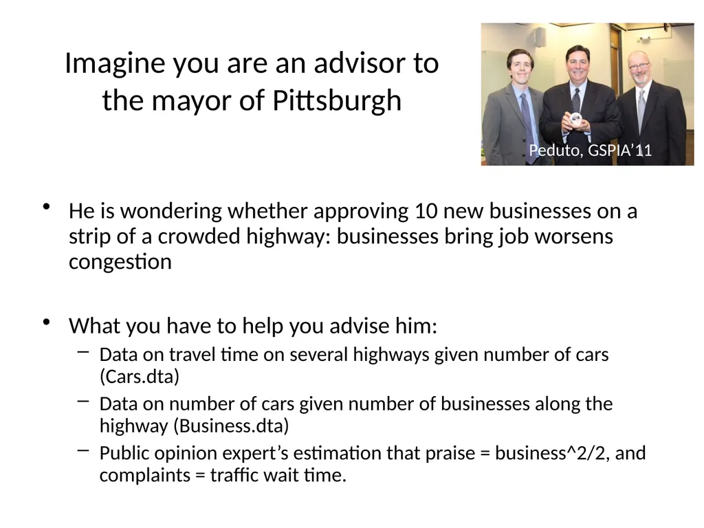
slide8. Imagine you are an advisor to the mayor of Pittsburgh He is wondering whether approving 10 new businesses on a strip of a crowded highway: businesses bring job worsens congestion

What you have to help you advise him:
Data on travel time on several highways given number of cars (Cars.dta)
Data on number of cars given number of businesses along the highway (Business.dta)
Public opinion expert’s estimation that praise = business^2/2, and complaints = traffic wait time. Peduto, GSPIA’11<br>
slide9. Breaking down the question into mathematical concepts how long does it take to travel the highway? (random variable)
how does the # of cars affect travel time? (correlation, linear regression, slope)
can adoption of a different traffic system reduce congestion? (simultaneous equations)
how does the # of businesses affect # of cars?(nonlinear equations)
what is the optimal # of business to have? (optimization)<br>
slide10. 1. random variable

How long does it take to travel through the highway?<br>
slide11. Random variable How long does it take to travel 20 miles on a city highway at 8am in the morning? Hands = 20 mins, 30 mins, 40 mins

Different day, same highway, same hour in day = different travel time.
Statistics is learning to get the information out of this uncertainty.
‘Time needed to travel’ is a random variable = the value is subject to variation due to chance.

Is what is written on this board ALL possible travel time for the 15 mile highway above? No. That would be the population. This is a sample. We usually only observe a sample of realizations of the random variable of interest.

Mean? Note also that if I had asked a different group of people, I would have written different numbers on the board, and therefore get a different mean.<br>
slide12. Looking at data Suppose cars.csv contains travel time and # of cars on various Pittsburgh highways
How do you load cars.csv into STATA so you can look at it?
We’ll do it 2 ways today, using the “Data Editor” and using the “insheet” command.
In general we’ll use STATA in two ways today, first using the drop down menu, and then using code.

Loading with Data Editor. Open cars.csv in Excel. Highlight, copy. Open data editor. Click on first cell and paste. Treat first row as variable name.

Note that the STATA you will learn today is just quick and dirty. You will learn how to use it properly in Quant I (with Jeremy) and Quant II (with me).<br>
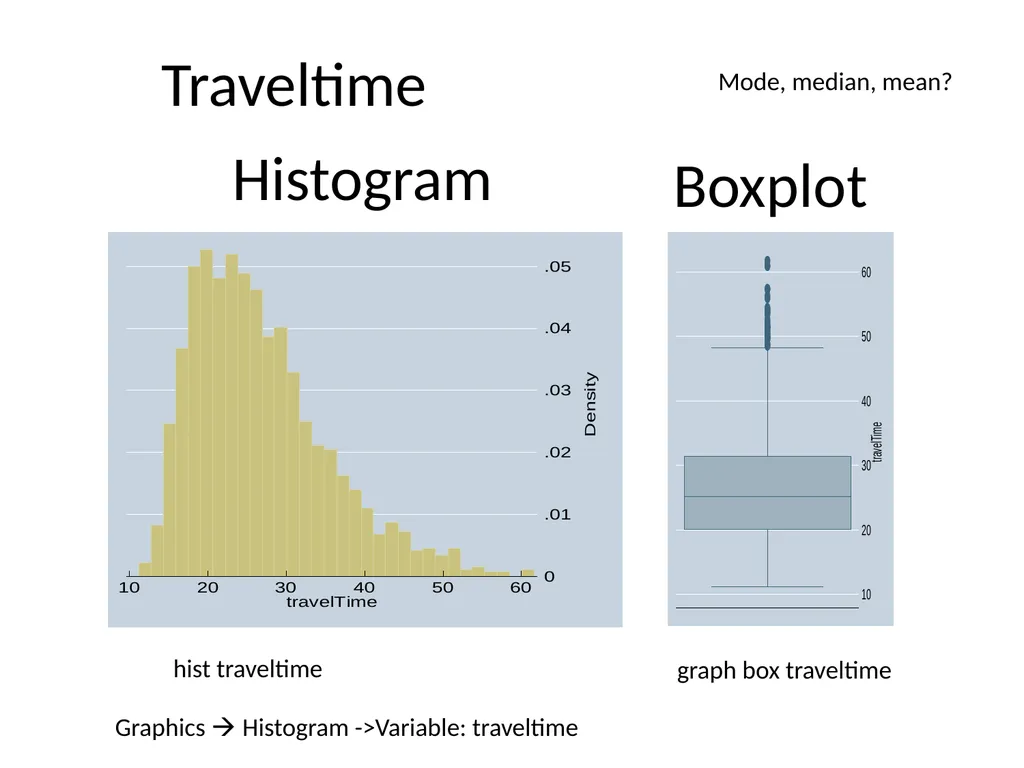
slide13. Histogram Boxplot Traveltime graph box traveltime hist traveltime Graphics  Histogram ->Variable: traveltime Mode, median, mean?<br>
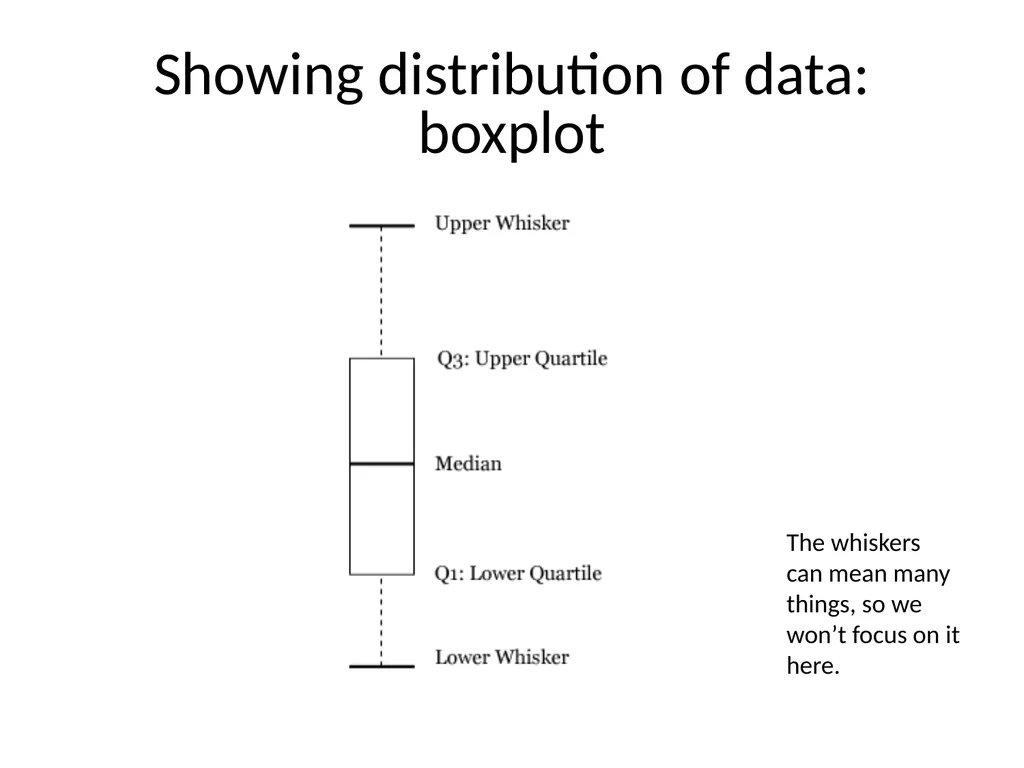
slide14. Showing distribution of data: boxplot The whiskers can mean many things, so we won’t focus on it here.<br>
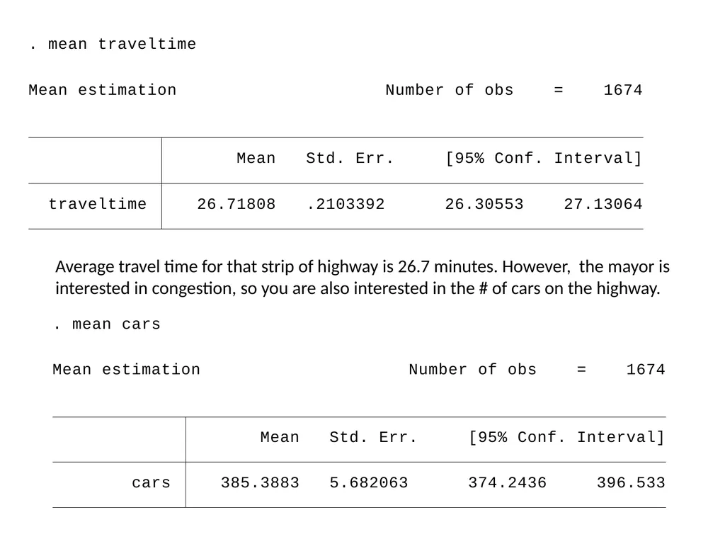
slide15. Average travel time for that strip of highway is 26.7 minutes. However, the mayor is interested in congestion, so you are also interested in the # of cars on the highway.<br>
slide16. # of cars on the highway Histogram Boxplot Hmm.. does this help you understand traffic congestion?<br>
slide17. 2. correlation, linear regression, slope / rate / derivative

how does the # of cars affect travel time?<br>
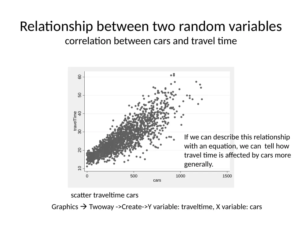
slide18. Relationship between two random variablescorrelation between cars and travel time If we can describe this relationship with an equation, we can tell how travel time is affected by cars more generally. scatter traveltime cars Graphics  Twoway ->Create->Y variable: traveltime, X variable: cars<br>
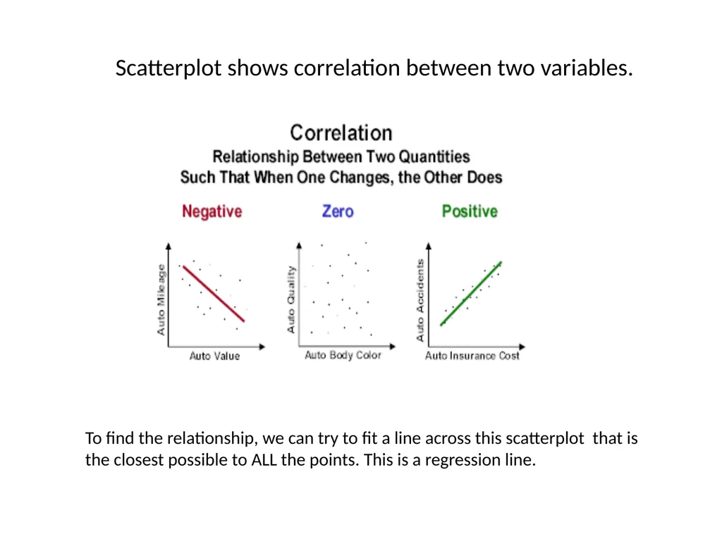
slide19. To find the relationship, we can try to fit a line across this scatterplot that is the closest possible to ALL the points. This is a regression line. Scatterplot shows correlation between two variables.<br>
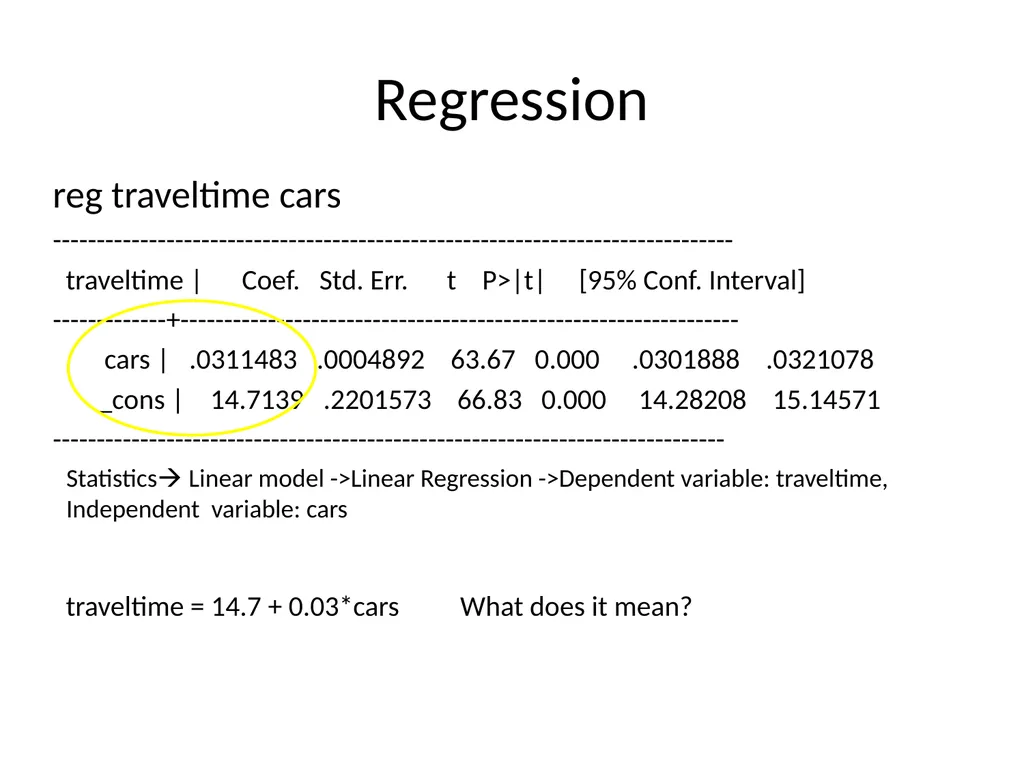
slide20. Regression traveltime = 14.7 + 0.03*cars What does it mean? reg traveltime cars
------------------------------------------------------------------------------
traveltime | Coef. Std. Err. t P>|t| [95% Conf. Interval]
-------------+----------------------------------------------------------------
cars | .0311483 .0004892 63.67 0.000 .0301888 .0321078
_cons | 14.7139 .2201573 66.83 0.000 14.28208 15.14571
----------------------------------------------------------------------------- Statistics Linear model ->Linear Regression ->Dependent variable: traveltime,
Independent variable: cars<br>
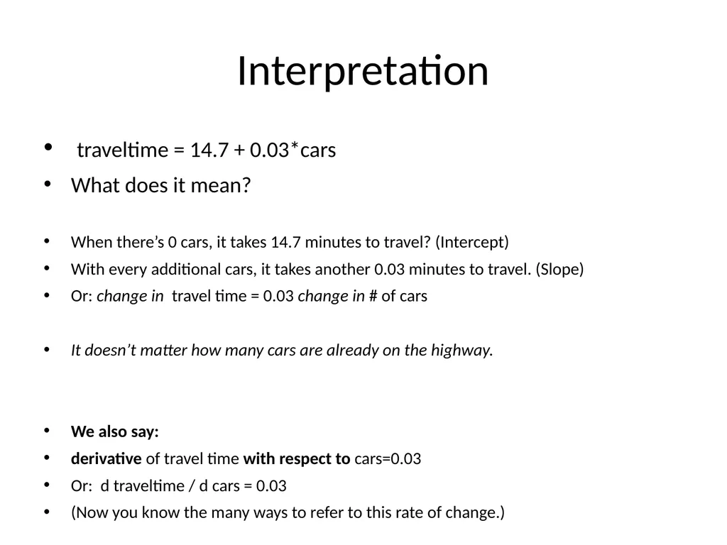
slide21. Interpretation traveltime = 14.7 + 0.03*cars
What does it mean?

When there’s 0 cars, it takes 14.7 minutes to travel? (Intercept)
With every additional cars, it takes another 0.03 minutes to travel. (Slope)
Or: change in travel time = 0.03 change in # of cars

It doesn’t matter how many cars are already on the highway.

We also say:
derivative of travel time with respect to cars=0.03
Or: d traveltime / d cars = 0.03
(Now you know the many ways to refer to this rate of change.)<br>
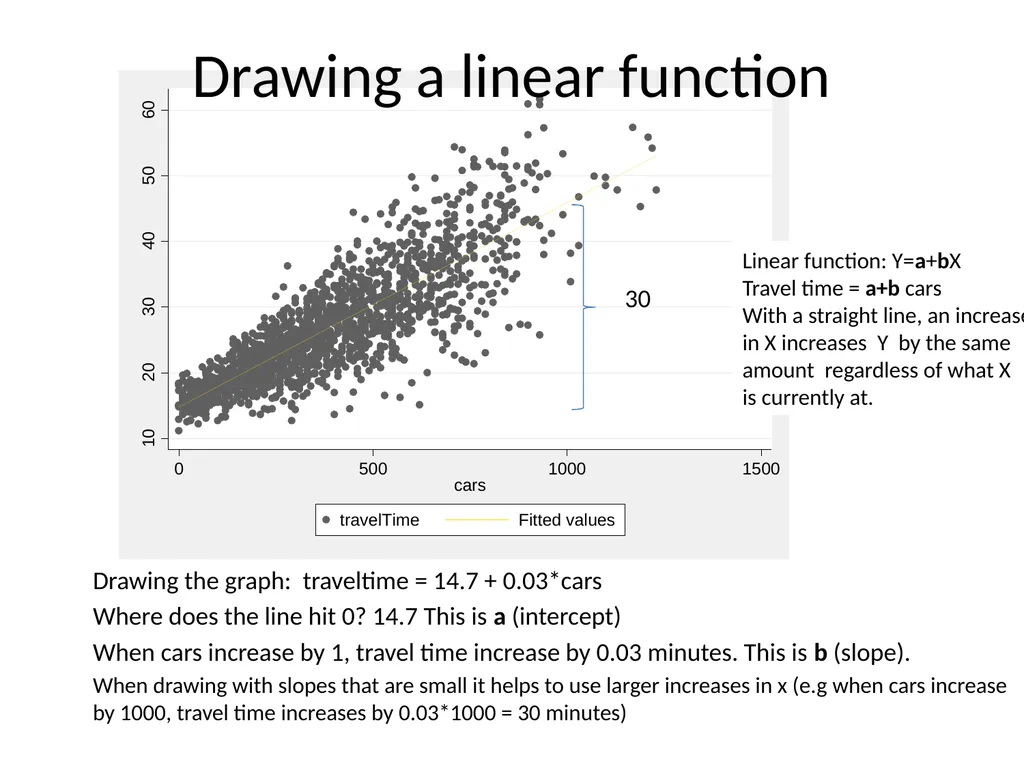
slide22. Drawing the graph:  traveltime = 14.7 + 0.03*cars
Where does the line hit 0? 14.7 This is a (intercept)
When cars increase by 1, travel time increase by 0.03 minutes. This is b (slope).
When drawing with slopes that are small it helps to use larger increases in x (e.g when cars increase by 1000, travel time increases by 0.03*1000 = 30 minutes) Linear function: Y=a+bX
Travel time = a+b cars
With a straight line, an increase
in X increases Y by the same
amount regardless of what X
is currently at. 30 Drawing a linear function<br>
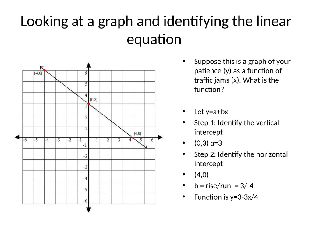
slide23. Looking at a graph and identifying the linear equation Suppose this is a graph of your patience (y) as a function of traffic jams (x). What is the function?

Let y=a+bx
Step 1: Identify the vertical intercept
(0,3) a=3
Step 2: Identify the horizontal intercept
(4,0)
b = rise/run = 3/-4
Function is y=3-3x/4<br>
slide24. Inverting a linear function traveltime = 14.7 + 0.03*cars
If it takes you 20 minutes to travel, how many cars are on a freeway?<br>
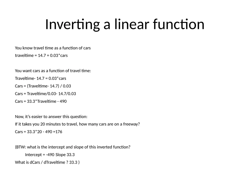
slide25. Inverting a linear function You know travel time as a function of cars
traveltime = 14.7 + 0.03*cars

You want cars as a function of travel time:
Traveltime- 14.7 = 0.03*cars
Cars = (Traveltime- 14.7) / 0.03
Cars = Traveltime/0.03- 14.7/0.03
Cars = 33.3*Traveltime - 490

Now, it’s easier to answer this question:
If it takes you 20 minutes to travel, how many cars are on a freeway?
Cars = 33.3*20 - 490 =176

(BTW: what is the intercept and slope of this inverted function?
Intercept = -490 Slope 33.3
What is dCars / dTraveltime ? 33.3 )<br>
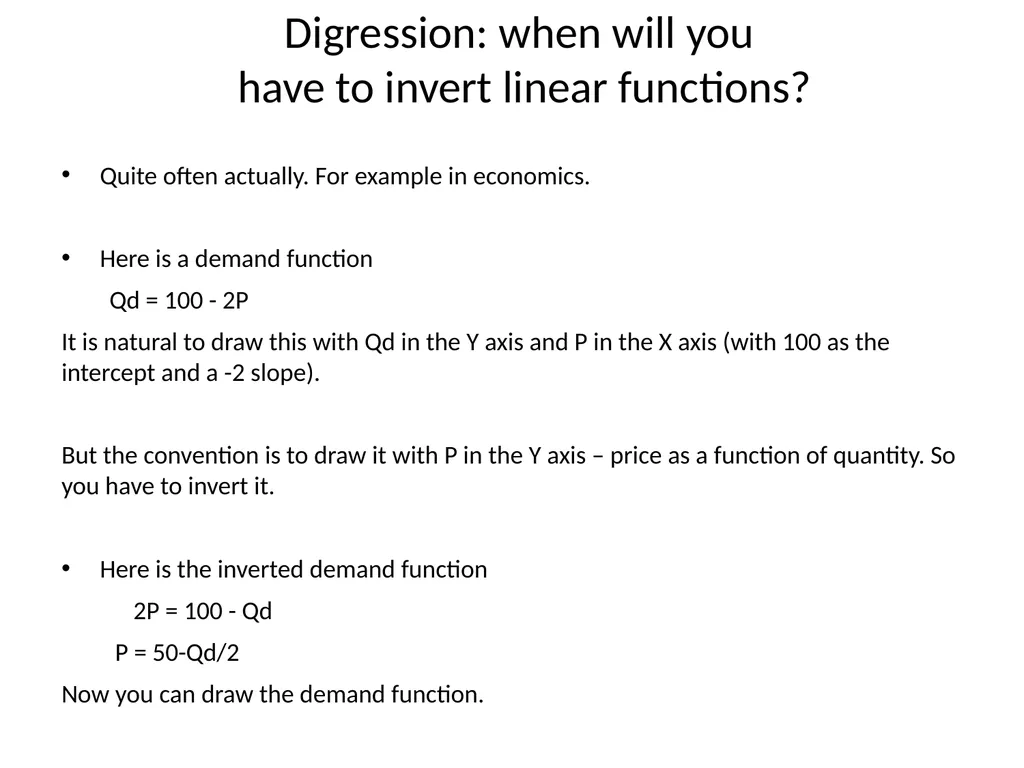
slide26. Digression: when will you have to invert linear functions? Quite often actually. For example in economics.

Here is a demand function
Qd = 100 - 2P
It is natural to draw this with Qd in the Y axis and P in the X axis (with 100 as the intercept and a -2 slope).

But the convention is to draw it with P in the Y axis – price as a function of quantity. So you have to invert it.

Here is the inverted demand function
2P = 100 - Qd
P = 50-Qd/2
Now you can draw the demand function.<br>
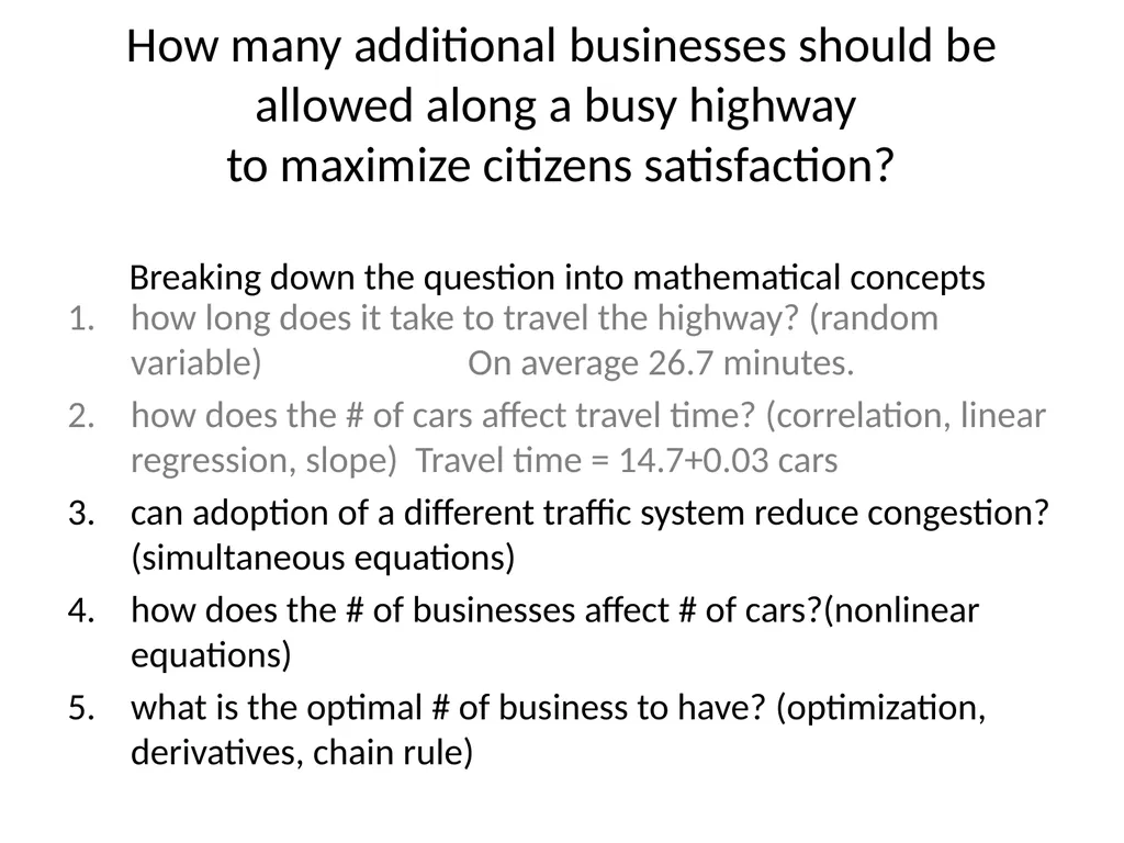
slide27. How many additional businesses should be allowed along a busy highway to maximize citizens satisfaction? Breaking down the question into mathematical concepts how long does it take to travel the highway? (random variable) On average 26.7 minutes.
how does the # of cars affect travel time? (correlation, linear regression, slope) Travel time = 14.7+0.03 cars
can adoption of a different traffic system reduce congestion? (simultaneous equations)
how does the # of businesses affect # of cars?(nonlinear equations)
what is the optimal # of business to have? (optimization, derivatives, chain rule)<br>
slide28. 3. comparing two highways: should you adopt another traffic system?

(simultaneous equations, or, systems of equations)<br>
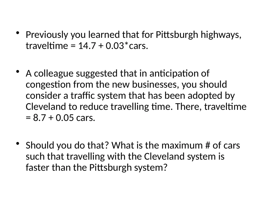
slide29. Previously you learned that for Pittsburgh highways, traveltime = 14.7 + 0.03*cars.

A colleague suggested that in anticipation of congestion from the new businesses, you should consider a traffic system that has been adopted by Cleveland to reduce travelling time. There, traveltime = 8.7 + 0.05 cars.

Should you do that? What is the maximum # of cars such that travelling with the Cleveland system is faster than the Pittsburgh system?<br>
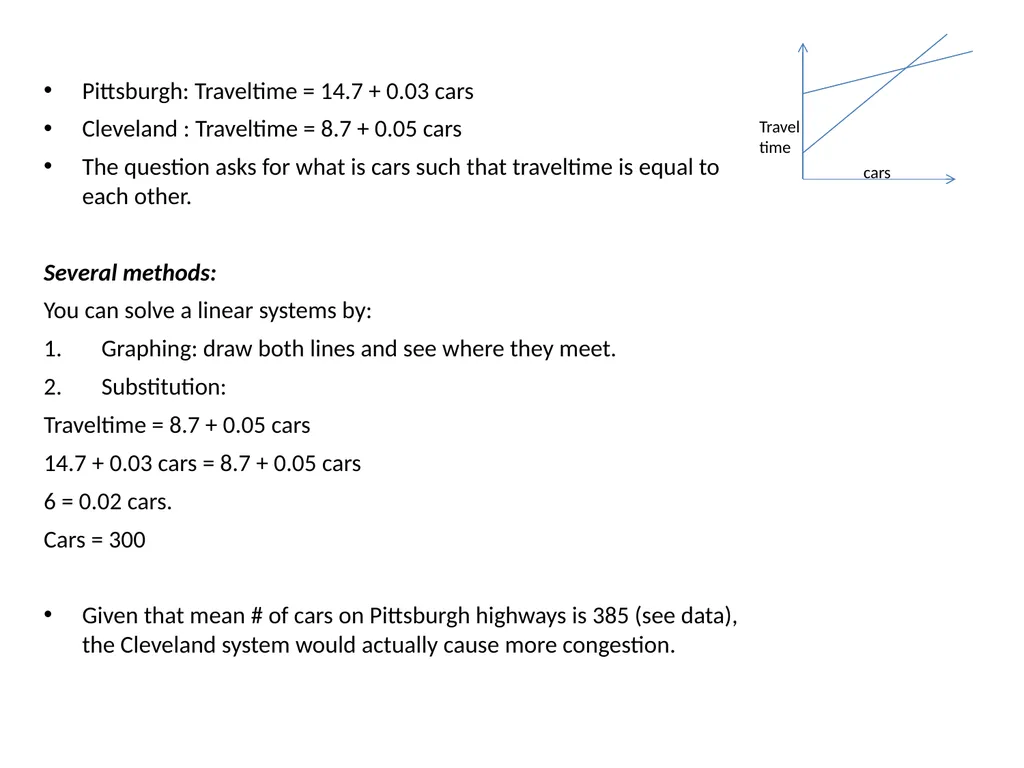
slide30. Pittsburgh: Traveltime = 14.7 + 0.03 cars
Cleveland : Traveltime = 8.7 + 0.05 cars
The question asks for what is cars such that traveltime is equal to each other.

Several methods:
You can solve a linear systems by:
Graphing: draw both lines and see where they meet.
Substitution:
Traveltime = 8.7 + 0.05 cars
14.7 + 0.03 cars = 8.7 + 0.05 cars
6 = 0.02 cars.
Cars = 300

Given that mean # of cars on Pittsburgh highways is 385 (see data), the Cleveland system would actually cause more congestion. Travel
time cars<br>
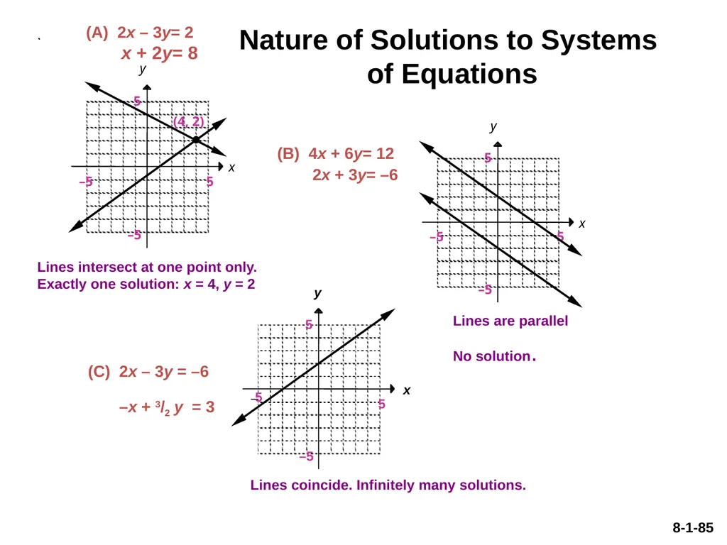
slide31. x y 5 –5 5 –5 (4, 2) x y 5 –5 5 –5 x y 5 – 5 5 –5 (A) 2x – 3y= 2
x + 2y= 8 (B) 4x + 6y= 12
2x + 3y= –6 Lines intersect at one point only.
Exactly one solution: x = 4, y = 2 Lines are parallel
No solution. (C) 2x – 3y = –6
–x + 3/2 y = 3 Lines coincide. Infinitely many solutions. Nature of Solutions to Systems
of Equations 8-1-85<br>
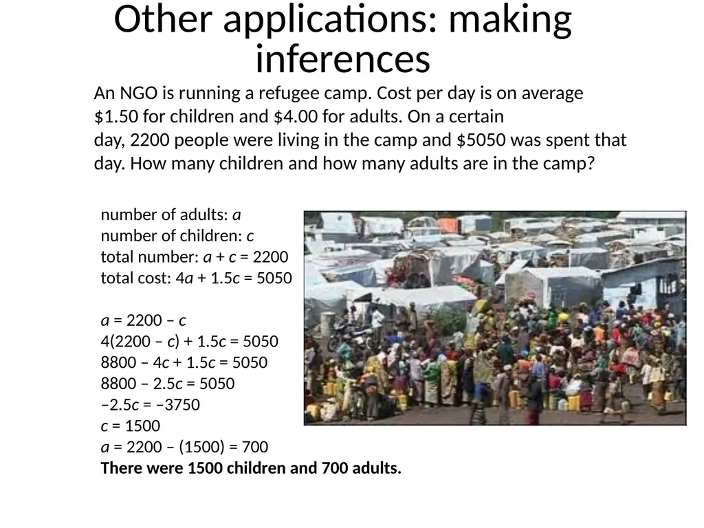
slide32. Other applications: making inferences An NGO is running a refugee camp. Cost per day is on average $1.50 for children and $4.00 for adults. On a certain day, 2200 people were living in the camp and $5050 was spent that day. How many children and how many adults are in the camp? number of adults: anumber of children: c
total number: a + c = 2200 total cost: 4a + 1.5c = 5050

a = 2200 – c
4(2200 – c) + 1.5c = 5050 8800 – 4c + 1.5c = 5050 8800 – 2.5c = 5050 –2.5c = –3750 c = 1500
a = 2200 – (1500) = 700
There were 1500 children and 700 adults.<br>
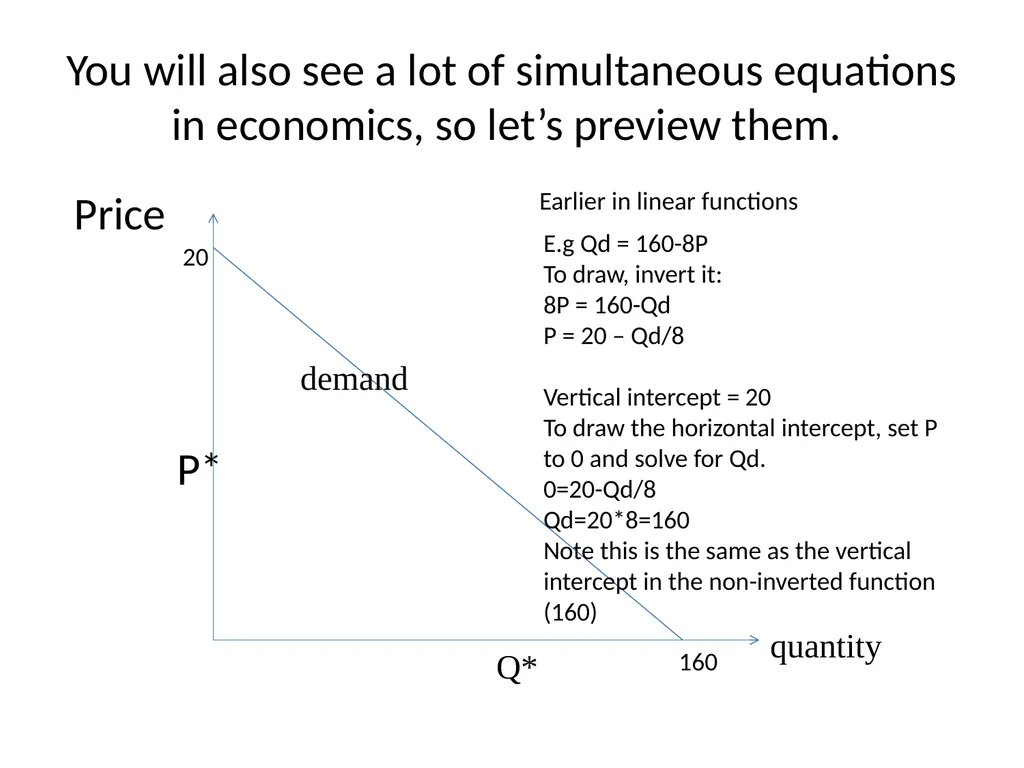
slide33. You will also see a lot of simultaneous equations in economics, so let’s preview them. Price

P* demand quantity Q* Earlier in linear functions E.g Qd = 160-8P
To draw, invert it:
8P = 160-Qd
P = 20 – Qd/8

Vertical intercept = 20
To draw the horizontal intercept, set P to 0 and solve for Qd.
0=20-Qd/8
Qd=20*8=160
Note this is the same as the vertical intercept in the non-inverted function (160) 20 160<br>
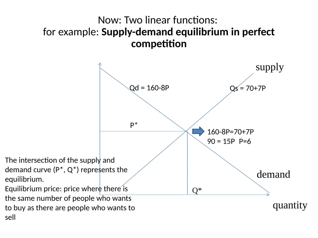
slide34. Now: Two linear functions: for example: Supply-demand equilibrium in perfect competition supply demand quantity Q* P* Qd = 160-8P Qs = 70+7P The intersection of the supply and demand curve (P*, Q*) represents the equilibrium.
Equilibrium price: price where there is the same number of people who wants to buy as there are people who wants to sell 160-8P=70+7P
90 = 15P P=6<br>
slide35. Exercise 1 10:15 am<br>
slide36. Alumni chat: Matt von Boecklin MPIA’13 More than Me Foundation, Liberia
Monitoring and Evaluation Manager – May 2015 - Present 
Project: Get REAL (Rebuild Education for All Liberians), a developing joint effort with the Ministry of Education to improve primary schools throughout Liberia. 
National Entrepreneurship Network (NEN), Bangalore, India
Entrepreneur Support and Impact Assessment Fellow — May 2014 – 2015 
Project: Dream to Destination Entrepreneur Support Program, a year-long intervention focusing on improving fundability, scalability, and revenue growth for 100 women-owned Indian enterprises.
Vital Voices Global Partnership, Washington D.C.
Program Evaluation Consultant — February - May 2014
Data Analysis Coordinator — June 2013 - January 2014
Project: Vital Voices Global Leadership Awards Program, an annual, weeklong event meant to enhance the credibility and visibility of extraordinary women leaders from around the world.<br>
slide37. 15 minutes breakWhen we return (11am) :Review Exercise 1Linear functions<br>
slide38. Review Exercise 1 Questions?<br>
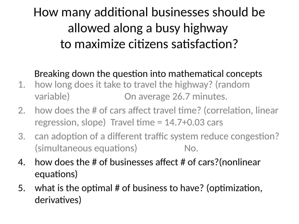
slide39. How many additional businesses should be allowed along a busy highway to maximize citizens satisfaction? Breaking down the question into mathematical concepts how long does it take to travel the highway? (random variable) On average 26.7 minutes.
how does the # of cars affect travel time? (correlation, linear regression, slope) Travel time = 14.7+0.03 cars
can adoption of a different traffic system reduce congestion? (simultaneous equations) No.
how does the # of businesses affect # of cars?(nonlinear equations)
what is the optimal # of business to have? (optimization, derivatives)<br>
slide40. 4. Nonlinear function We will now use our other data set, “business.csv”
This data set has # of businesses on a highway and the number of commuter cars associated with these businesses. what would new businesses do to highway congestion?<br>
slide41. clear (you must clear out the old data)
Load new Business.csv
Look in data editor

What relationship are we trying to figure out?<br>
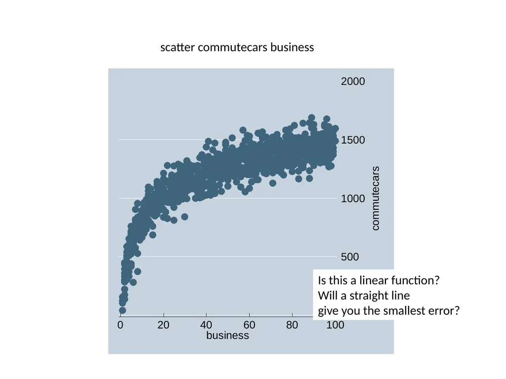
slide42. Is this a linear function?
Will a straight line
give you the smallest error? scatter commutecars business<br>
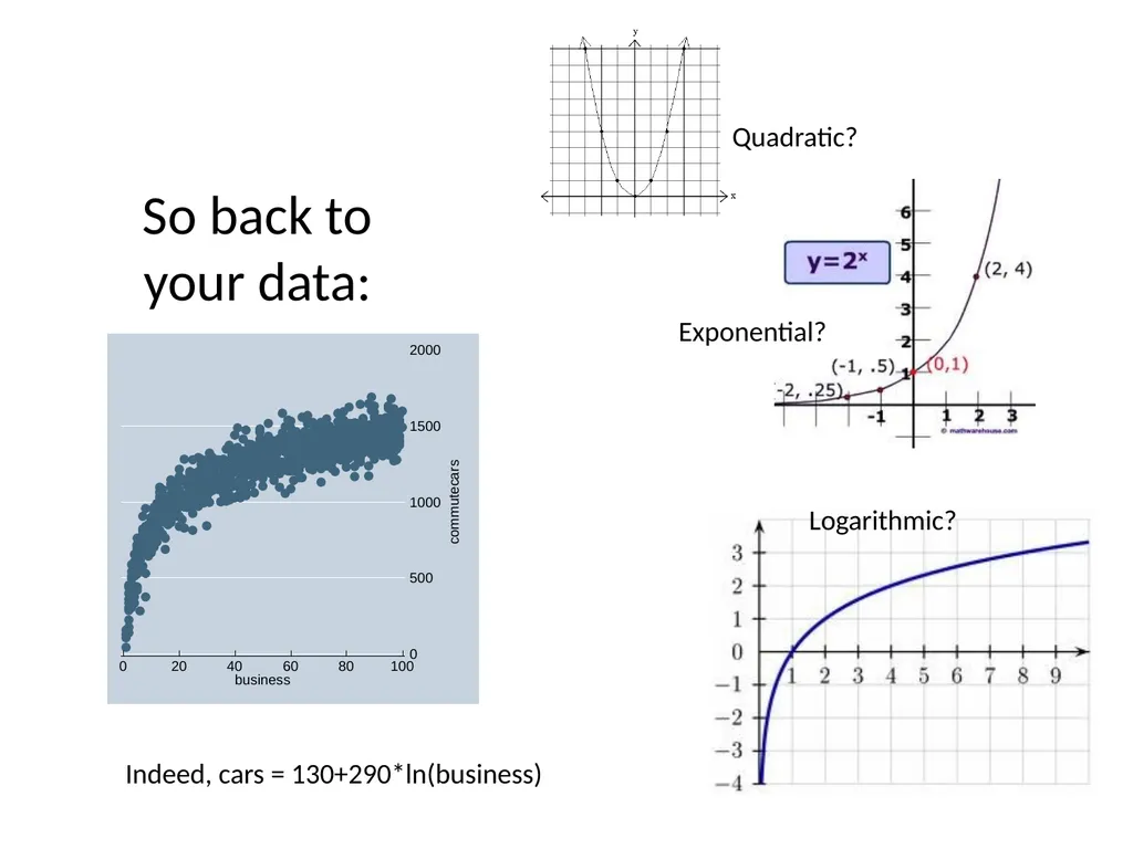
slide43. Nonlinear functions Let’s find what our function resembles:
Quadratic function
Logarithmic function
Exponential function<br>
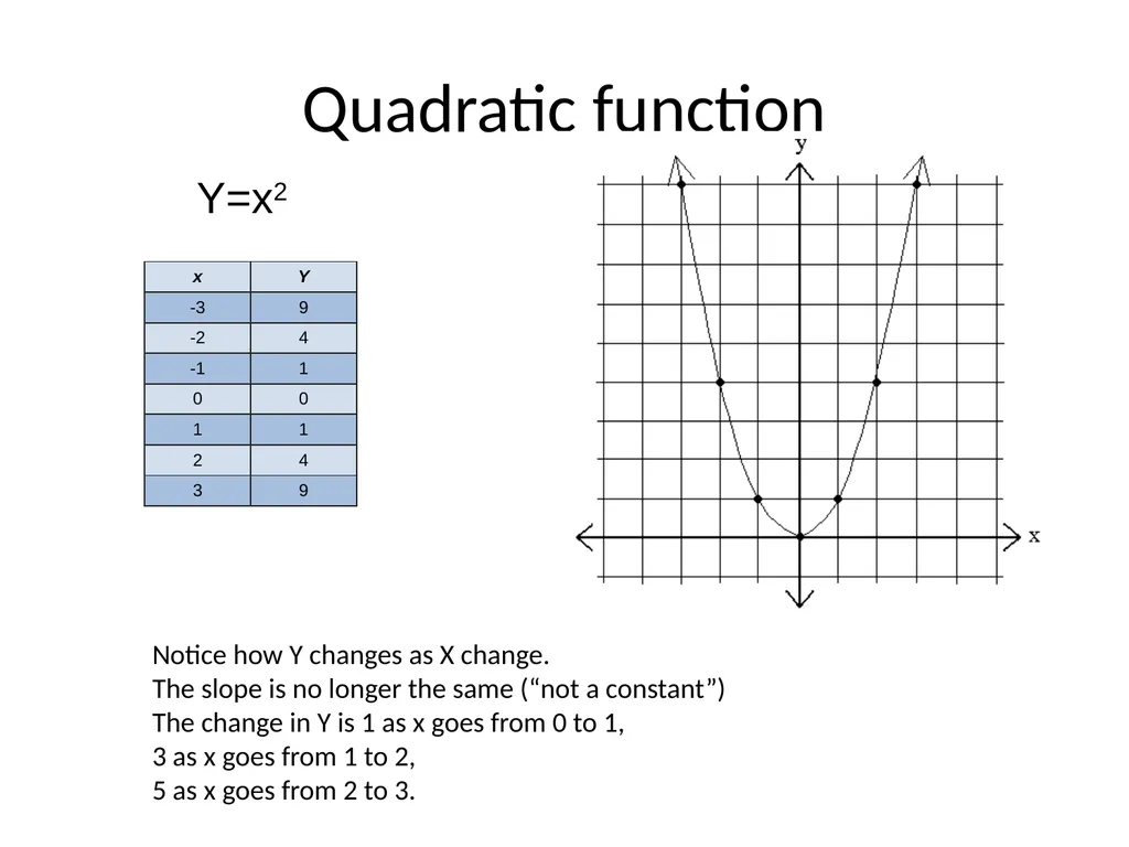
slide44. Quadratic function Y=x2 Notice how Y changes as X change.
The slope is no longer the same (“not a constant”)
The change in Y is 1 as x goes from 0 to 1,
3 as x goes from 1 to 2,
5 as x goes from 2 to 3.<br>
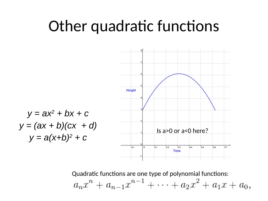
slide45. Other quadratic functions Is a>0 or a<0 here? Quadratic functions are one type of polynomial functions:<br>
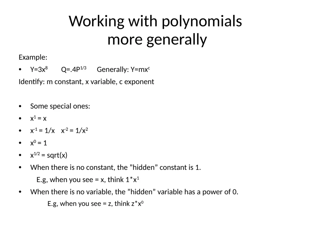
slide46. Working with polynomials more generally Example:
Y=3x8 Q=.4P1/3 Generally: Y=mxc
Identify: m constant, x variable, c exponent

Some special ones:
x1 = x
x-1 = 1/x x-2 = 1/x2
x0 = 1
x1/2 = sqrt(x)
When there is no constant, the ”hidden” constant is 1.
E.g, when you see = x, think 1*x1
When there is no variable, the ”hidden” variable has a power of 0.
E.g, when you see = z, think z*x0<br>
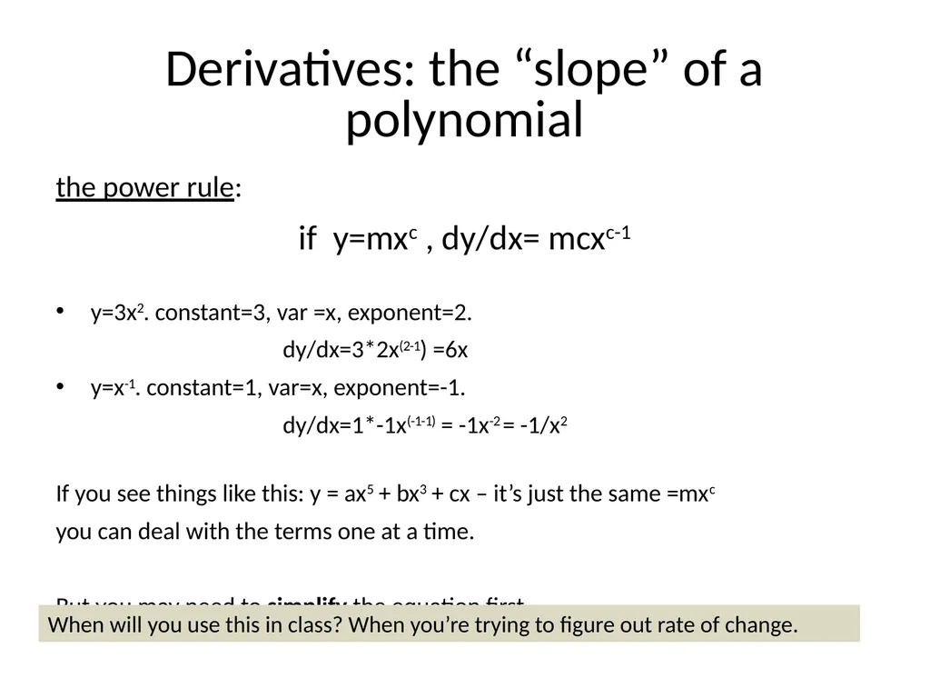
slide47. Derivatives: the “slope” of a polynomial the power rule:
if y=mxc , dy/dx= mcxc-1

y=3x2. constant=3, var =x, exponent=2.
dy/dx=3*2x(2-1) =6x
y=x-1. constant=1, var=x, exponent=-1.
dy/dx=1*-1x(-1-1) = -1x-2 = -1/x2

If you see things like this: y = ax5 + bx3 + cx – it’s just the same =mxc
you can deal with the terms one at a time.

But you may need to simplify the equation first. When will you use this in class? When you’re trying to figure out rate of change.<br>
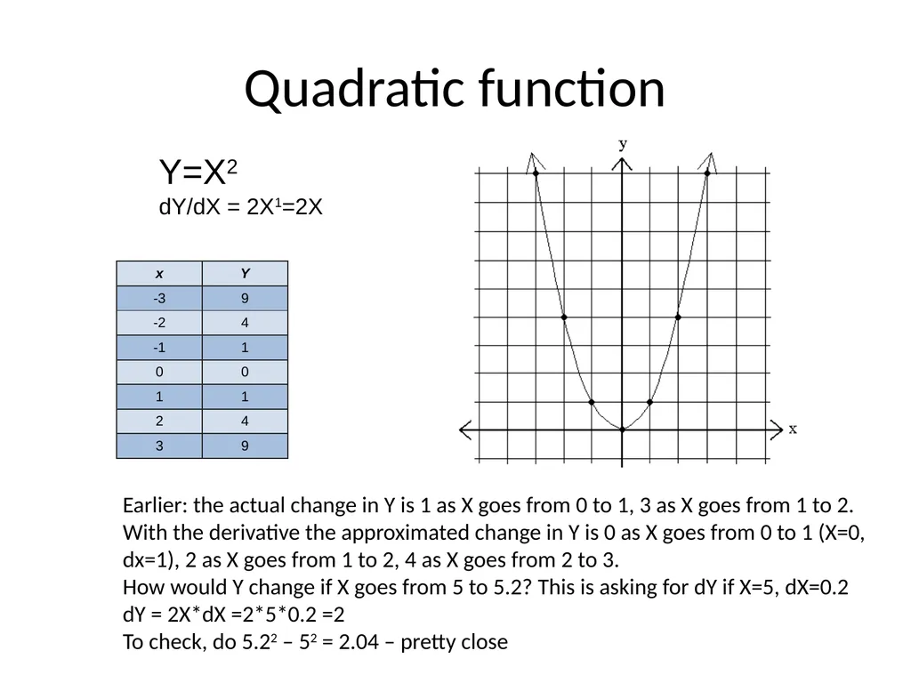
slide48. Quadratic function Y=X2
dY/dX = 2X1=2X Earlier: the actual change in Y is 1 as X goes from 0 to 1, 3 as X goes from 1 to 2.
With the derivative the approximated change in Y is 0 as X goes from 0 to 1 (X=0, dx=1), 2 as X goes from 1 to 2, 4 as X goes from 2 to 3.
How would Y change if X goes from 5 to 5.2? This is asking for dY if X=5, dX=0.2
dY = 2X*dX =2*5*0.2 =2
To check, do 5.22 – 52 = 2.04 – pretty close<br>
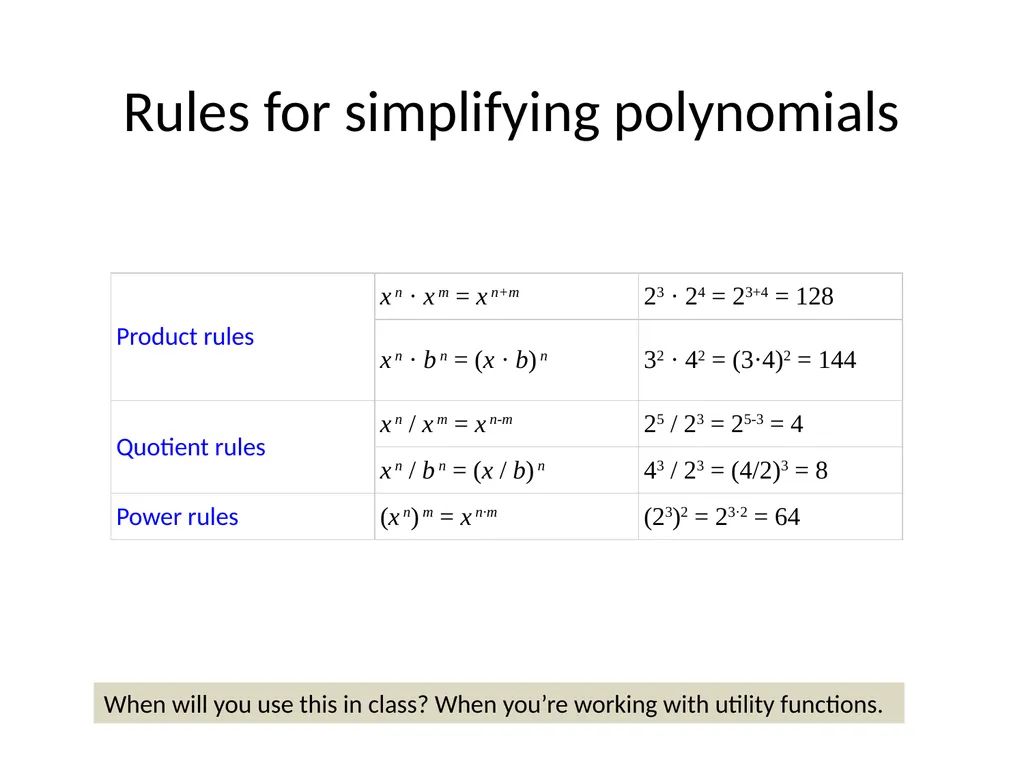
slide49. Rules for simplifying polynomials When will you use this in class? When you’re working with utility functions.<br>
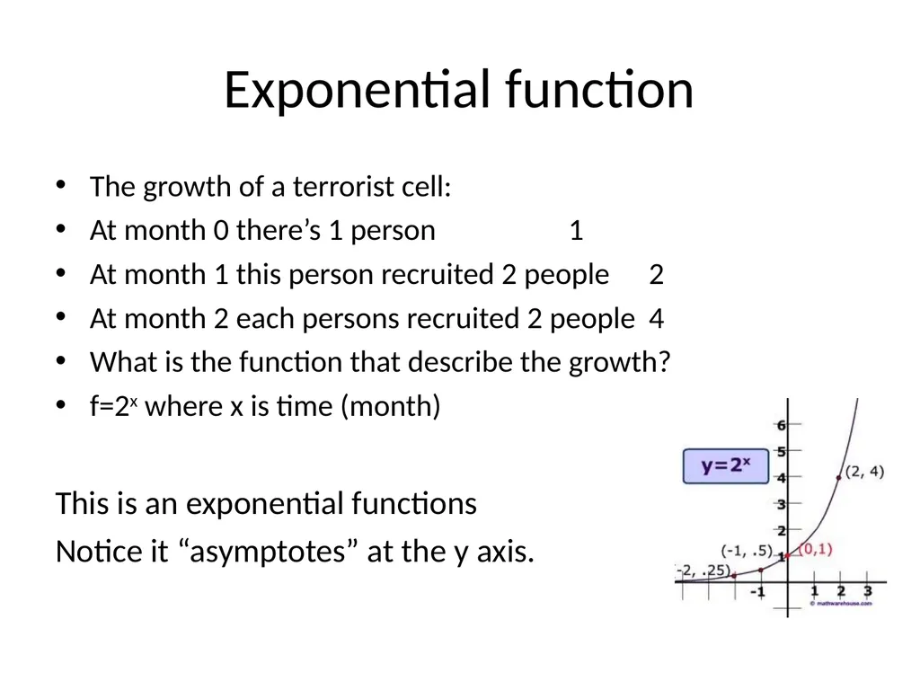
slide50. Exponential function The growth of a terrorist cell:
At month 0 there’s 1 person 1
At month 1 this person recruited 2 people 2
At month 2 each persons recruited 2 people 4
What is the function that describe the growth?
f=2x where x is time (month)

This is an exponential functions
Notice it “asymptotes” at the y axis.<br>
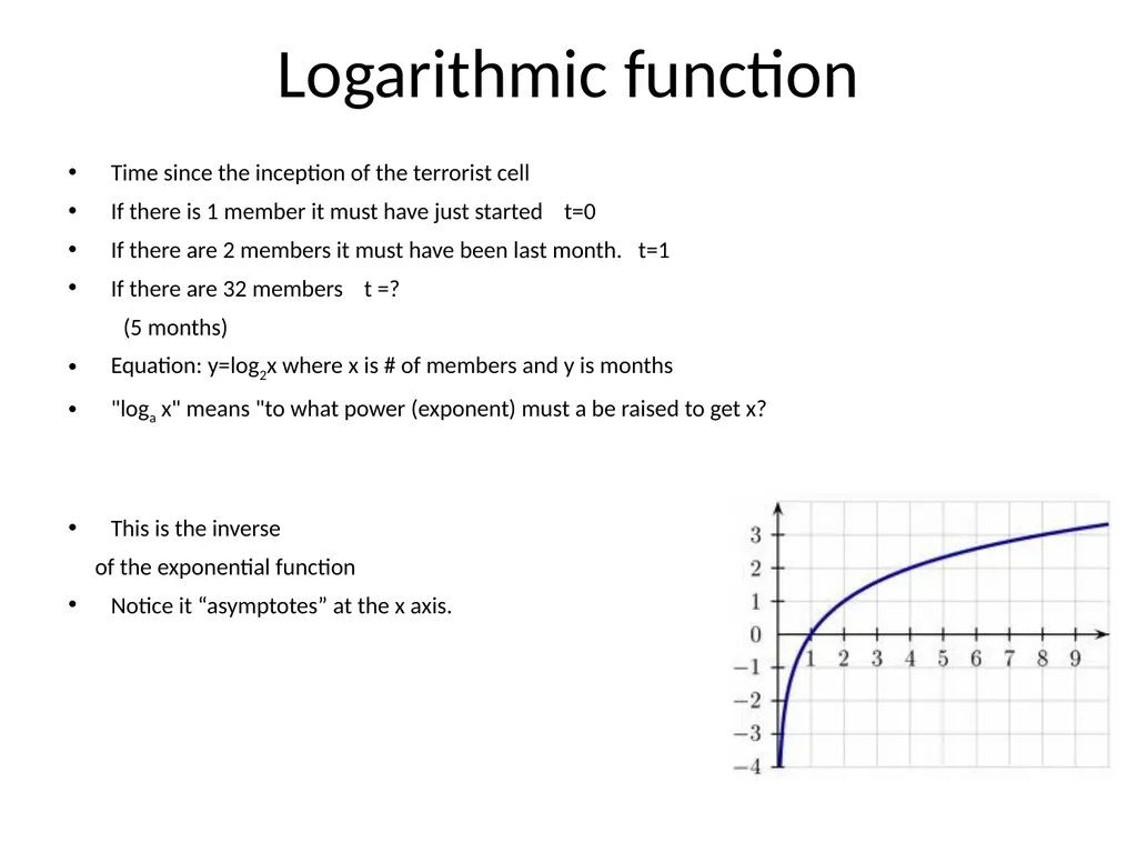
slide51. Logarithmic function Time since the inception of the terrorist cell
If there is 1 member it must have just started t=0
If there are 2 members it must have been last month. t=1
If there are 32 members t =?
(5 months)
Equation: y=log2x where x is # of members and y is months
"loga x" means "to what power (exponent) must a be raised to get x?

This is the inverse
of the exponential function
Notice it “asymptotes” at the x axis.<br>
slide52. 2x and exp(x)Logs and natural logs Exp(x) = 2.72x
This quantity is often used when quantities grow proportionally to it’s value. It is often seen in math, physics, and chemistry. When will you use this? When you’re learning about logistic regressions.<br>
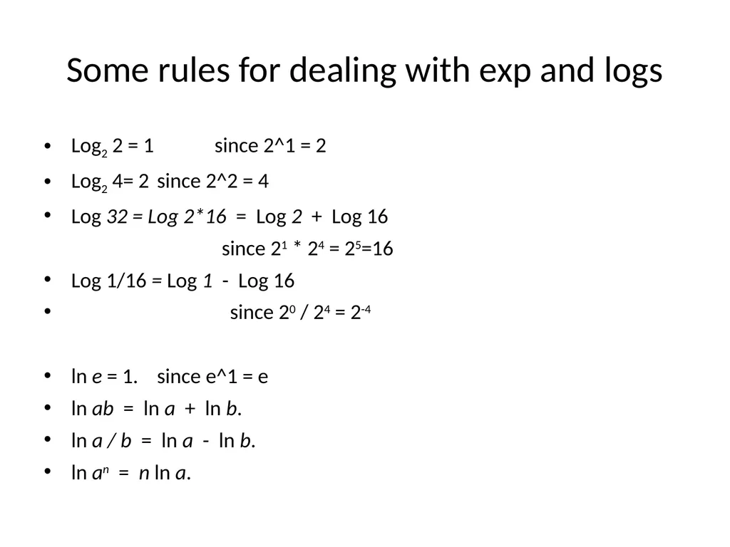
slide53. Some rules for dealing with exp and logs Log2 2 = 1 since 2^1 = 2
Log2 4= 2 since 2^2 = 4
Log 32 = Log 2*16  =  Log 2  +  Log 16
since 21 * 24 = 25=16
Log 1/16 = Log 1  -  Log 16
since 20 / 24 = 2-4

ln e = 1. since e^1 = e
ln ab  =  ln a  +  ln b.
ln a / b  =  ln a  -  ln b.
ln an  =  n ln a.<br>
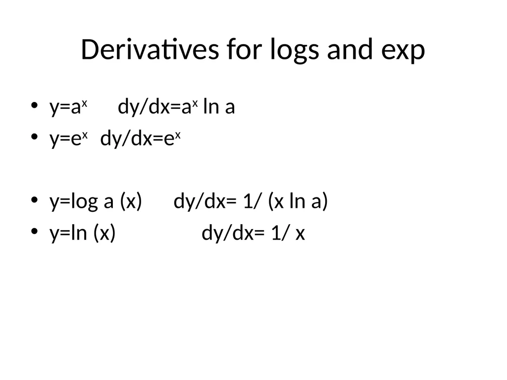
slide54. Derivatives for logs and exp y=ax dy/dx=ax ln a
y=ex dy/dx=ex

y=log a (x) dy/dx= 1/ (x ln a)
y=ln (x) dy/dx= 1/ x<br>
slide55. Exponential? Logarithmic? Quadratic? So back to your data: Indeed, cars = 130+290*ln(business)<br>
slide56. 5. what is the optimal # of business to have? (optimization, compound functions)<br>
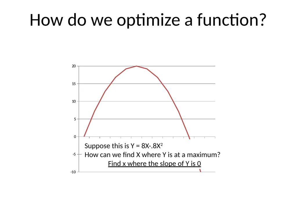
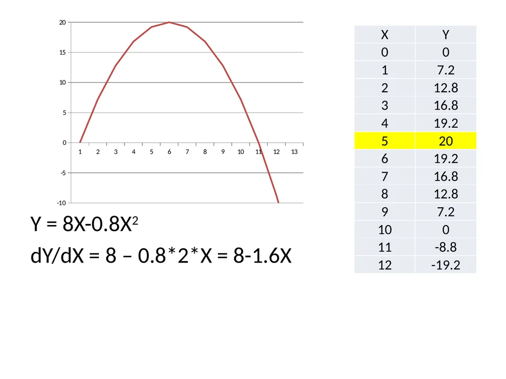
slide57. How do we optimize a function? Suppose this is Y = 8X-.8X2
How can we find X where Y is at a maximum?
Find x where the slope of Y is 0<br>
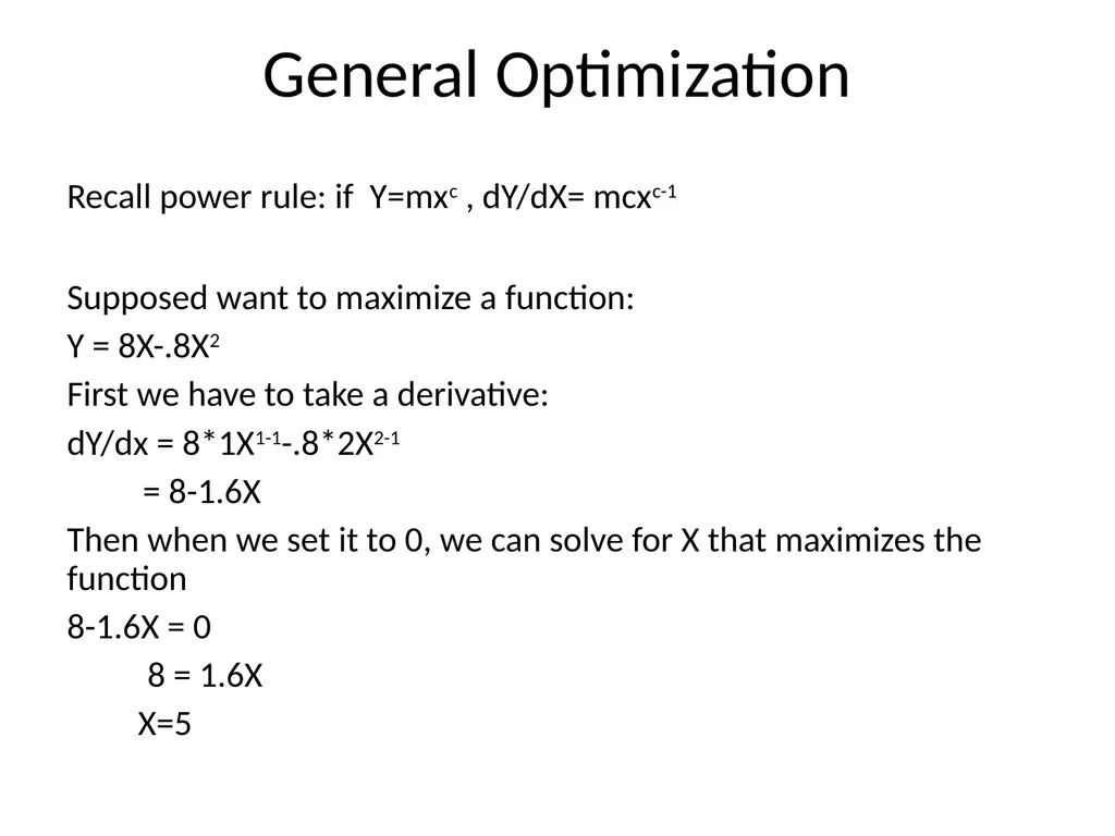
slide58. General Optimization Recall power rule: if Y=mxc , dY/dX= mcxc-1

Supposed want to maximize a function:
Y = 8X-.8X2
First we have to take a derivative:
dY/dx = 8*1X1-1-.8*2X2-1
= 8-1.6X
Then when we set it to 0, we can solve for X that maximizes the function
8-1.6X = 0
8 = 1.6X
X=5<br>
slide59. Y = 8X-0.8X2
dY/dX = 8 – 0.8*2*X = 8-1.6X<br>
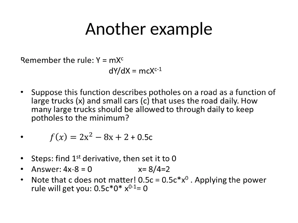
slide60. Another example<br>
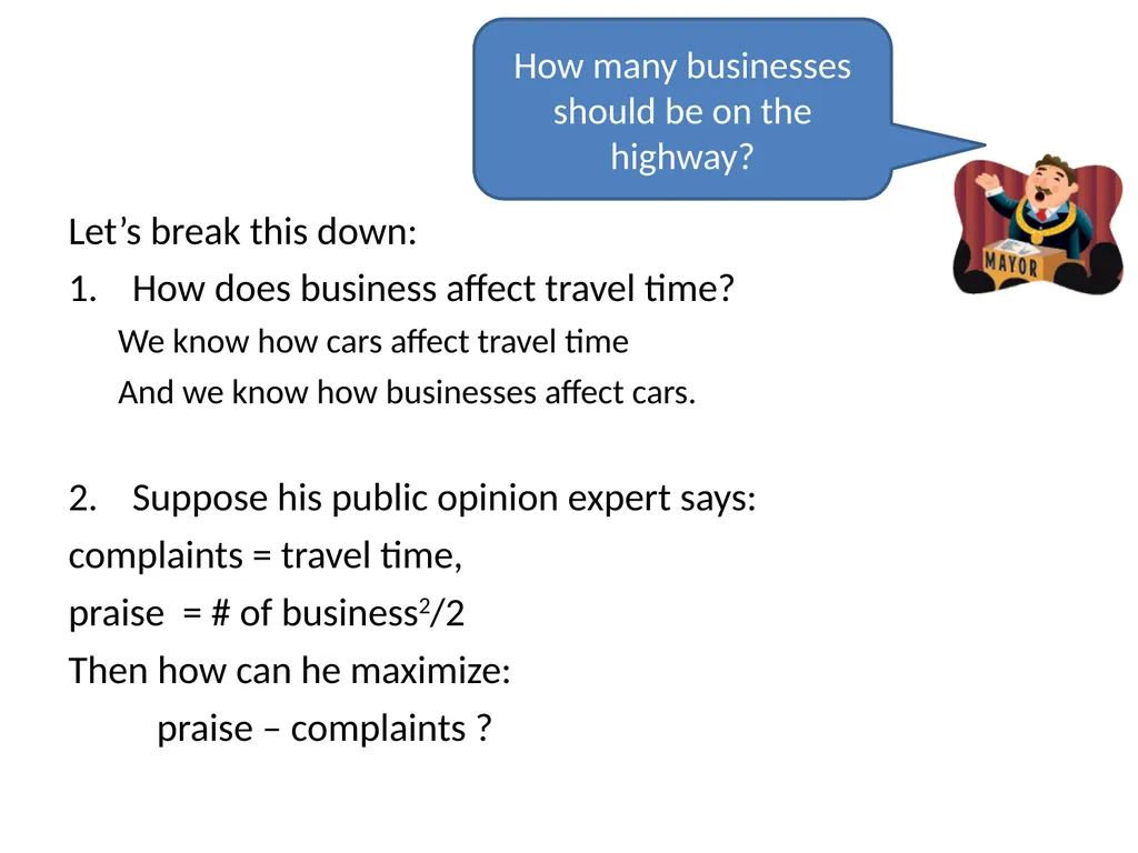
slide61. Let’s break this down:
How does business affect travel time?
We know how cars affect travel time
And we know how businesses affect cars.

Suppose his public opinion expert says:
complaints = travel time,
praise = # of business2/2
Then how can he maximize:
praise – complaints ? How many businesses should be on the highway?<br>
slide62. You have cars and traveltime. You have business and cars. How do you combine them?

cars = 130+290*ln(business)
traveltime = 14.7 + 0.03*cars
traveltime = 14.7 + 0.03* (130+290*ln(business) )
traveltime = 18.6+8.7ln(business)

How does an additional business affect travel time?
dt/db = 8.7/business
If there’s 1 business on the highway, 1 extra business will add 8.7/1 = 8.7 minutes to traffic
If there are 100, 1 extra will add 8.7/100 = 0.087 minutes to traffic

How does a small business (treat this as db=0.5) affect travel time?
Change in t = (8.7 /business) change in b
If there’s 1 business on the highway, 0.5 extra business will add (8.7/1)*0.5 = 4.35 minutes to traffic<br>
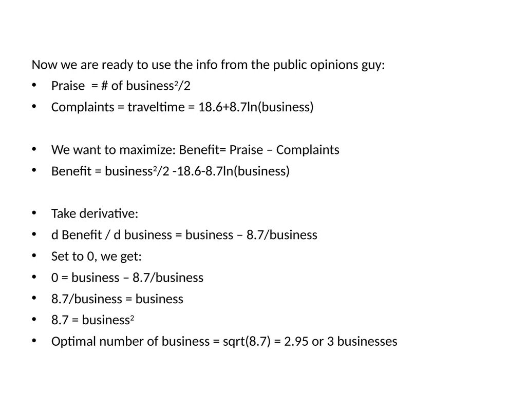
slide63. Now we are ready to use the info from the public opinions guy:
Praise = # of business2/2
Complaints = traveltime = 18.6+8.7ln(business)

We want to maximize: Benefit= Praise – Complaints
Benefit = business2/2 -18.6-8.7ln(business)

Take derivative:
d Benefit / d business = business – 8.7/business
Set to 0, we get:
0 = business – 8.7/business
8.7/business = business
8.7 = business2
Optimal number of business = sqrt(8.7) = 2.95 or 3 businesses<br>
slide64. Exercise 2 12:30 lunch come back 1:30pm<br>
slide65. 1:30 Review Exercise 2 Any questions?<br>
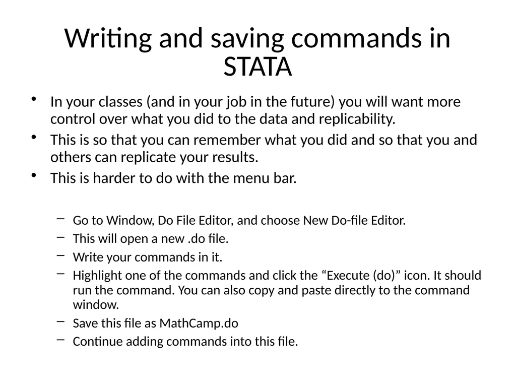
slide66. Writing and saving commands in STATA In your classes (and in your job in the future) you will want more control over what you did to the data and replicability.
This is so that you can remember what you did and so that you and others can replicate your results.
This is harder to do with the menu bar.

Go to Window, Do File Editor, and choose New Do-file Editor.
This will open a new .do file.
Write your commands in it.
Highlight one of the commands and click the “Execute (do)” icon. It should run the command. You can also copy and paste directly to the command window.
Save this file as MathCamp.do
Continue adding commands into this file.<br>
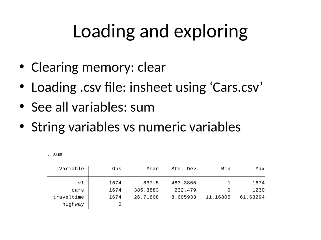
slide67. Loading and exploring Clearing memory: clear
Loading .csv file: insheet using ‘Cars.csv’
See all variables: sum
String variables vs numeric variables<br>
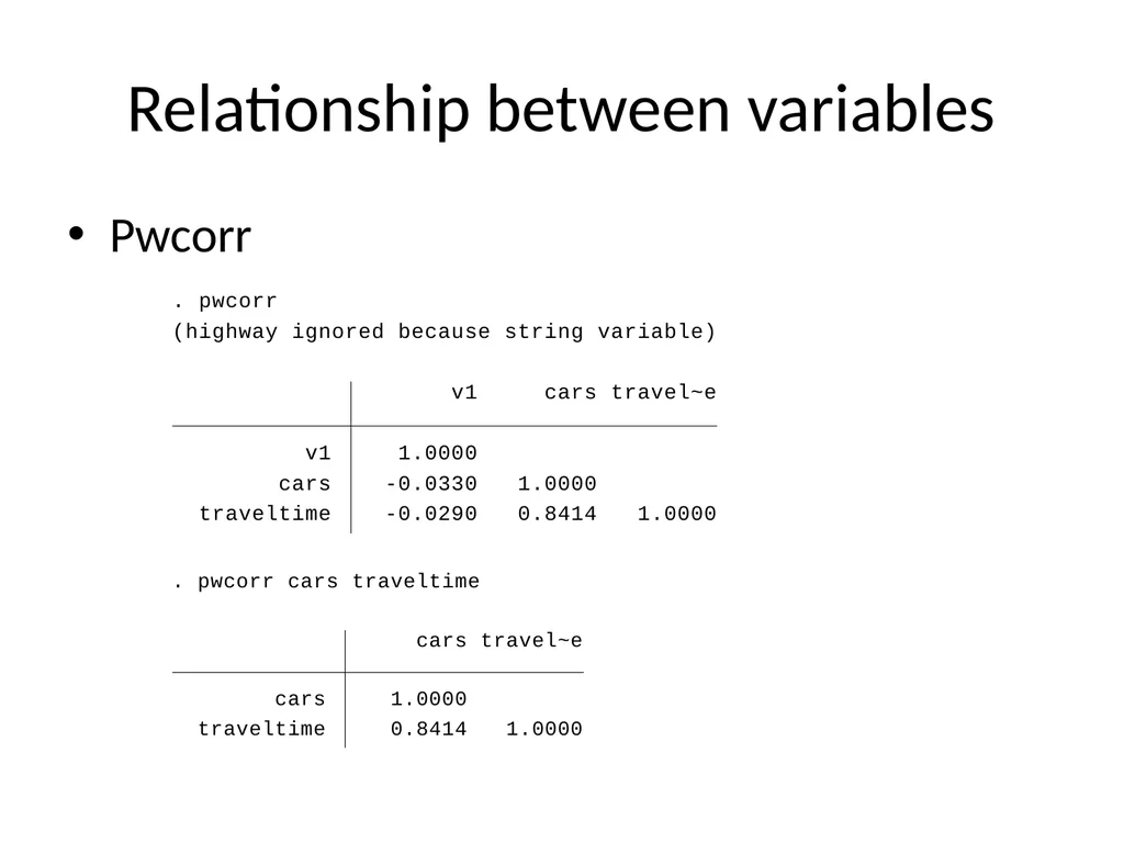
slide68. Relationship between variables Pwcorr<br>
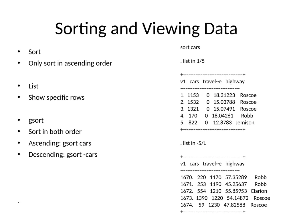
slide69. Sorting and Viewing Data Sort
Only sort in ascending order

List
Show specific rows

gsort
Sort in both order
Ascending: gsort cars
Descending: gsort -cars

. sort cars

. list in 1/5

+----------------------------------+
v1 cars travel~e highway
----------------------------------
1. 1153 0 18.31223 Roscoe
2. 1532 0 15.03788 Roscoe
3. 1321 0 15.07491 Roscoe
4. 170 0 18.04261 Robb
5. 822 0 12.8783 Jemison
+----------------------------------+

. list in -5/L

+----------------------------------+
v1 cars travel~e highway
----------------------------------
1670. 220 1170 57.35289 Robb
1671. 253 1190 45.25637 Robb
1672. 554 1210 55.85953 Clarion
1673. 1390 1220 54.14872 Roscoe
1674. 59 1230 47.82588 Roscoe
+----------------------------------+<br>
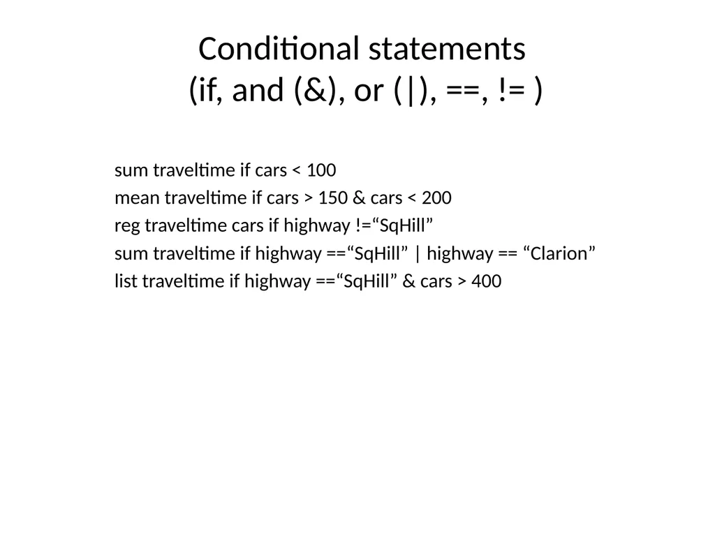
slide70. Conditional statements (if, and (&), or (|), ==, != ) sum traveltime if cars < 100
mean traveltime if cars > 150 & cars < 200
reg traveltime cars if highway !=“SqHill”
sum traveltime if highway ==“SqHill” | highway == “Clarion”
list traveltime if highway ==“SqHill” & cars > 400<br>
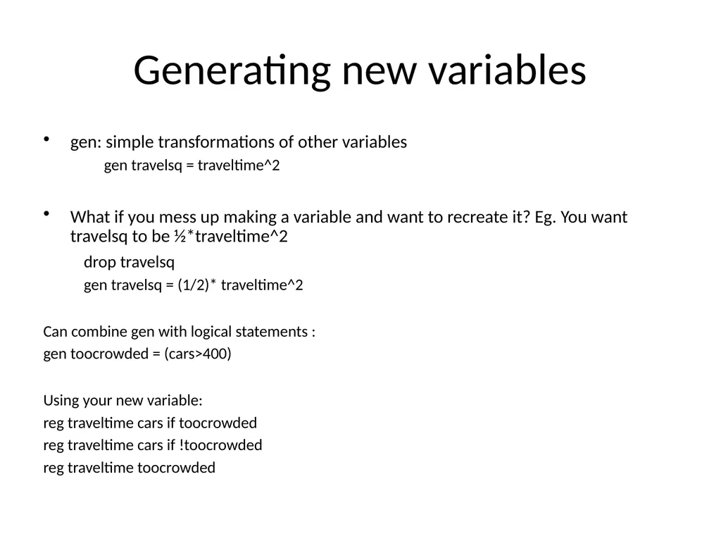
slide71. Generating new variables gen: simple transformations of other variables
gen travelsq = traveltime^2

What if you mess up making a variable and want to recreate it? Eg. You want travelsq to be ½*traveltime^2
drop travelsq
gen travelsq = (1/2)* traveltime^2

Can combine gen with logical statements :
gen toocrowded = (cars>400)

Using your new variable:
reg traveltime cars if toocrowded
reg traveltime cars if !toocrowded
reg traveltime toocrowded<br>
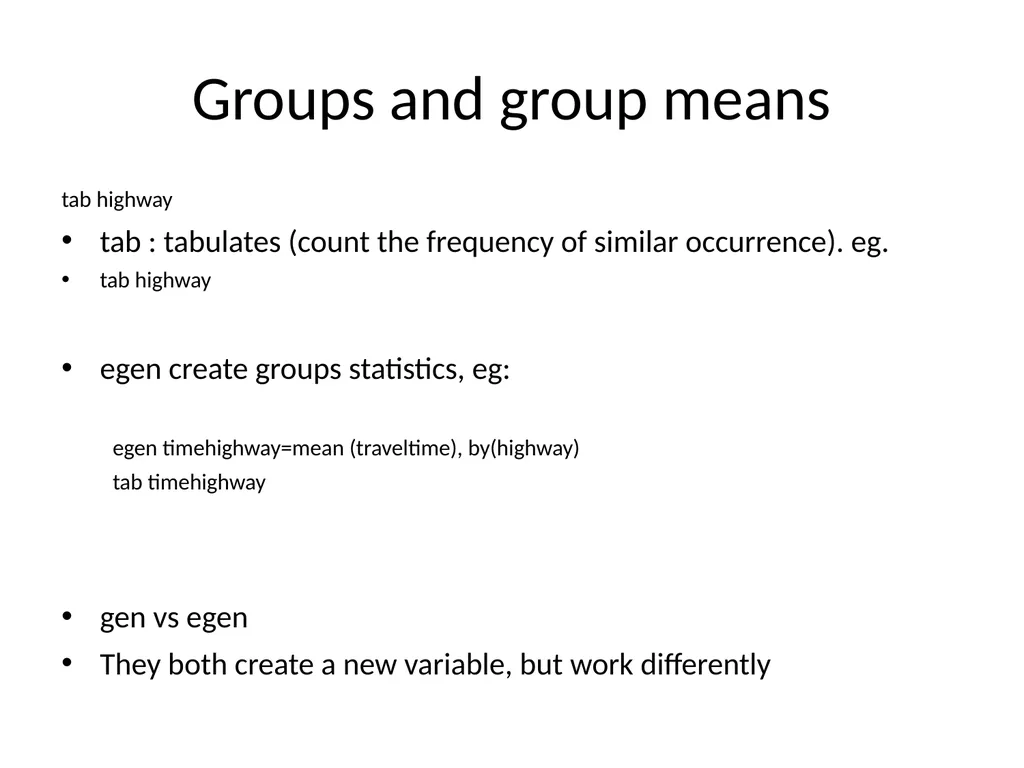
slide72. Groups and group means tab highway
tab : tabulates (count the frequency of similar occurrence). eg.
tab highway

egen create groups statistics, eg:

egen timehighway=mean (traveltime), by(highway)
tab timehighway

gen vs egen
They both create a new variable, but work differently<br>
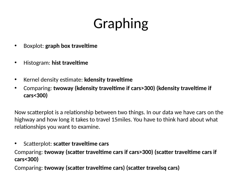
slide73. Graphing Boxplot: graph box traveltime

Histogram: hist traveltime

Kernel density estimate: kdensity traveltime
Comparing: twoway (kdensity traveltime if cars>300) (kdensity traveltime if cars<300)

Now scatterplot is a relationship between two things. In our data we have cars on the highway and how long it takes to travel 15miles. You have to think hard about what relationships you want to examine.

Scatterplot: scatter traveltime cars
Comparing: twoway (scatter traveltime cars if cars>300) (scatter traveltime cars if cars<300)
Comparing: twoway (scatter traveltime cars) (scatter travelsq cars)

How to save your graphs?
File– Save As – (I usually do .pdf)
Or: Win users: right click and click Copy and then paste into your word doc.

Try it.<br>
slide74. If have time: A little bit on how random variable vary and on statistical significanceElse:Exercise 3<br>
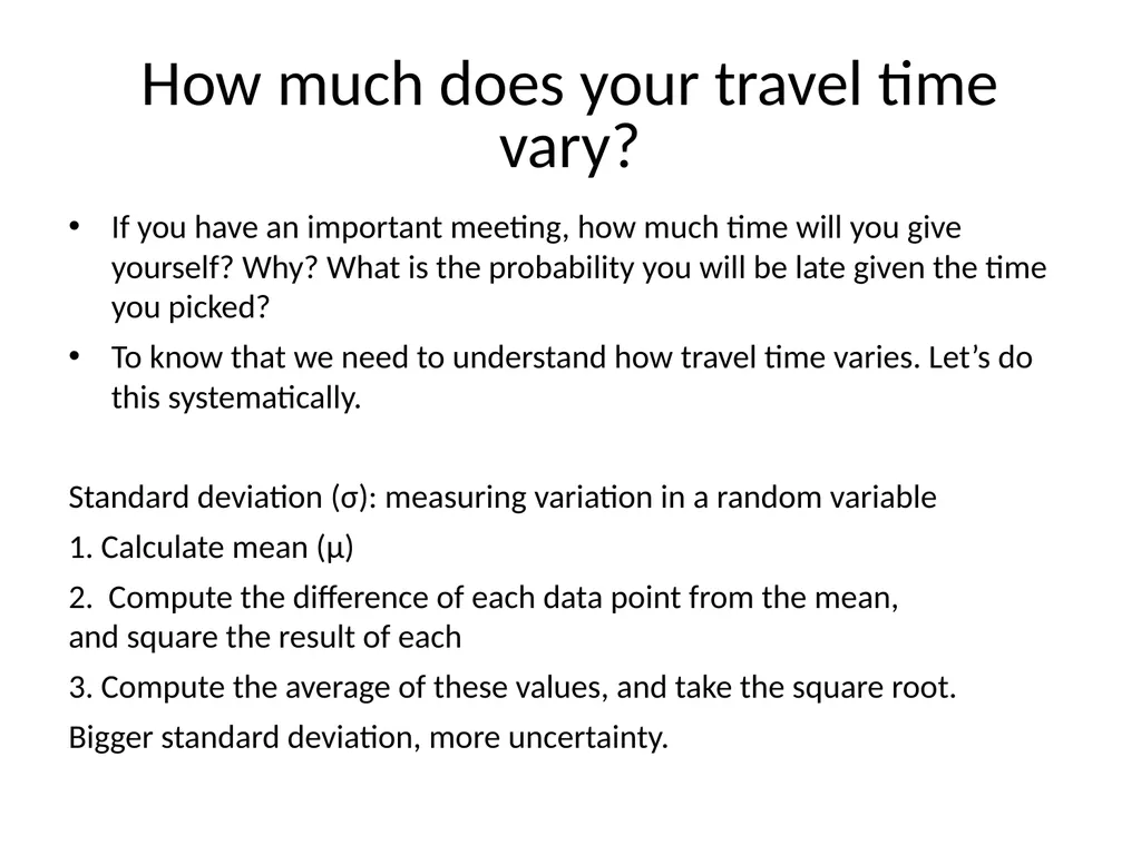
slide75. How much does your travel time vary? If you have an important meeting, how much time will you give yourself? Why? What is the probability you will be late given the time you picked?
To know that we need to understand how travel time varies. Let’s do this systematically.

Standard deviation (σ): measuring variation in a random variable
1. Calculate mean (μ)
2. Compute the difference of each data point from the mean, and square the result of each
3. Compute the average of these values, and take the square root.
Bigger standard deviation, more uncertainty.<br>
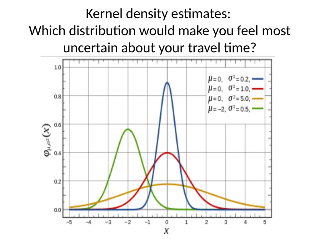
slide76. Kernel density estimates: Which distribution would make you feel most uncertain about your travel time?<br>
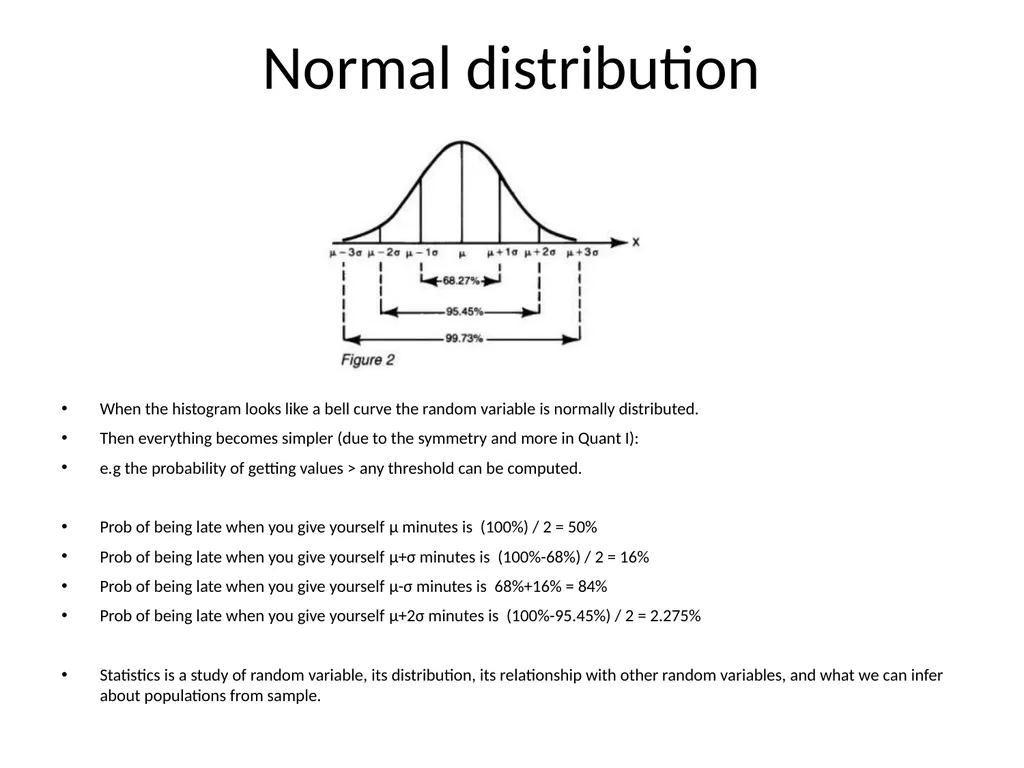
slide77. Normal distribution When the histogram looks like a bell curve the random variable is normally distributed.
Then everything becomes simpler (due to the symmetry and more in Quant I):
e.g the probability of getting values > any threshold can be computed.

Prob of being late when you give yourself μ minutes is (100%) / 2 = 50%
Prob of being late when you give yourself μ+σ minutes is (100%-68%) / 2 = 16%
Prob of being late when you give yourself μ-σ minutes is 68%+16% = 84%
Prob of being late when you give yourself μ+2σ minutes is (100%-95.45%) / 2 = 2.275%

Statistics is a study of random variable, its distribution, its relationship with other random variables, and what we can infer about populations from sample.<br>
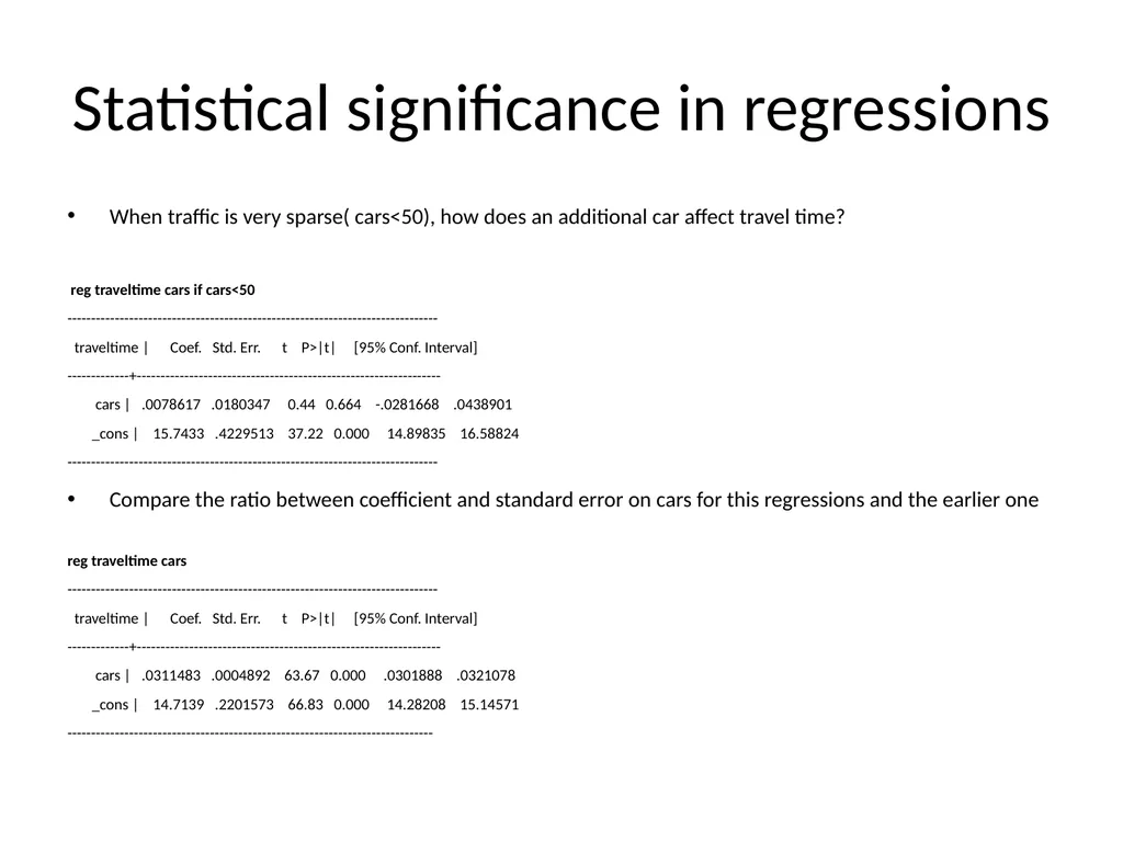
slide78. Statistical significance in regressions When traffic is very sparse( cars<50), how does an additional car affect travel time?

reg traveltime cars if cars<50
------------------------------------------------------------------------------
traveltime | Coef. Std. Err. t P>|t| [95% Conf. Interval]
-------------+----------------------------------------------------------------
cars | .0078617 .0180347 0.44 0.664 -.0281668 .0438901
_cons | 15.7433 .4229513 37.22 0.000 14.89835 16.58824
------------------------------------------------------------------------------
Compare the ratio between coefficient and standard error on cars for this regressions and the earlier one

reg traveltime cars
------------------------------------------------------------------------------
traveltime | Coef. Std. Err. t P>|t| [95% Conf. Interval]
-------------+----------------------------------------------------------------
cars | .0311483 .0004892 63.67 0.000 .0301888 .0321078
_cons | 14.7139 .2201573 66.83 0.000 14.28208 15.14571
-----------------------------------------------------------------------------<br>
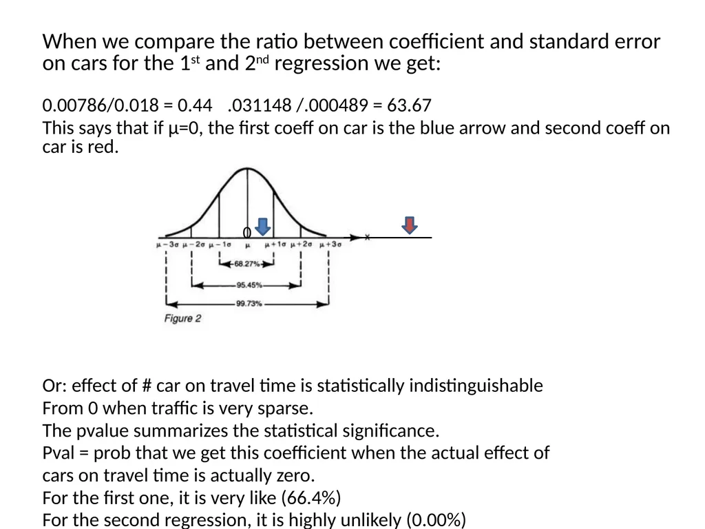
slide79. When we compare the ratio between coefficient and standard error on cars for the 1st and 2nd regression we get:

0.00786/0.018 = 0.44 .031148 /.000489 = 63.67
This says that if μ=0, the first coeff on car is the blue arrow and second coeff on car is red.

Or: effect of # car on travel time is statistically indistinguishable
From 0 when traffic is very sparse.
The pvalue summarizes the statistical significance.
Pval = prob that we get this coefficient when the actual effect of
cars on travel time is actually zero.
For the first one, it is very like (66.4%)
For the second regression, it is highly unlikely (0.00%)<br>
slide80. 2:45pm Faculty Chat

Jeremy Weber,
Assistant Professor of Economics
Will teach Intro to Quant
Previously Research Economist
at the U.S. Department of Agriculture

Michael Lewin,
Lecturer
Will be teaching Econ for Public Affairs
Previously Senior Economist
at the World Bank

Break 3:00 to chat informally with faculty, we start lecture at 3:30<br>
slide81. Review Exercise 3 Any questions?
On to teams.
We will call out your names. When you meet up you are going to move to sit together.
In the last exercise you will work together in your new team.<br>
slide82. On to the Race!Here are the teams Come up and meet your teammate as your name is called.

Show Race Packet Materials.
Tomorrow: you will absolutely need your computer.
You will be coding and thinking and racing from room to room, so make sure you are comfortable.
There will be 9 clues. Solving each clue under three tries will earn your team 1 point. The team with the highest number of points wins the race. Ties are broken by how quickly you complete the race.
There will be Roadblocks. In Roadblocks each person in the team must solve a puzzle individually. The point will only be given if both team members succesfully solve their puzzle.<br>
slide83. How to win? Review all the material tonight with your teammate and decide on how you want to handle roadblocks and other scenarios. The math will be simple but will require creative applications.
Stata commands: You MUST get familiar with all the commands we did today.
When getting your answers checked you can send just one person so one of you can continue working.
Tomorrow: you can setup starting from 8:30am. We will distribute materials for the race at 9am.
On to work with your teammate!<br>
slide84. Training done!<br>