
MANAGEMENT ACCOUNTING INTRODUCTION: A business



















Description: MANAGEMENT ACCOUNTING INTRODUCTION: A business enterprise must keep a systematic record of what happens from day- tot-day events so that it can know its position clearly. Most of the business enterprises are run by the corporate sector.
Related Topics
Download Presentation
"MANAGEMENT ACCOUNTING INTRODUCTION: A business" is the property of its rightful owner. Permission is granted to download and print the materials on this website for personal, non-commercial use only, and to display it on your personal computer provided you do not modify the materials and that you retain all copyright notices contained in the materials. By downloading content from our website, you accept the terms of this agreement.
Presentation Transcript
slide1. MANAGEMENT ACCOUNTING
INTRODUCTION:
A business enterprise must keep a systematic record of what happens from day- tot-day events so that it can know its position clearly. Most of the business enterprises are run by the corporate sector. These business houses are required by law to prepare periodical statements in proper form showing the state of financial affairs. The systematic record of the daily events of a business leading to presentation of a complete financial picture is known as accounting. Thus, Accounting is the language of business. A business enterprise speaks through accounting. It reveals the position, especially the financial position through the language called accounting.
MEANING OF ACCOUNTING:
Accounting is the process of recording, classifying, summarizing, analyzing and interpreting the financial transactions of the business for the benefit of management and those parties who are interested in business such as shareholders, creditors, bankers, customers, employees and government. Thus, it is concerned with financial reporting and decision making aspects of the business.
The American Institute of Certified Public Accountants Committee on Terminology proposed in 1941 that accounting may be defined as, “The art of recording, classifying and summarizing in a significant manner and in terms of money, transactions and events which are, in part at least, of a financial character and interpreting the results thereof”.<br>
slide2. BRANCHES OF ACCOUNTING:
Accounting can be classified into three categories:
Financial Accounting
Cost Accounting, and
Management Accounting
FINANCIAL ACCOUNTING:
The term „Accounting‟ unless otherwise specifically stated always refers to
„Financial Accounting‟. Financial Accounting is commonly carries on in the general offices of a business. It is concerned with revenues, expenses, assets and liabilities of a business house. Financial Accounting has two-fold objective, viz,
To ascertain the profitability of the business, and
To know the financial position of the concern.
NATURE AND SCOPE OF FINANCIAL ACCOUNTING:
Financial accounting is a useful tool to management and to external users such as shareholders, potential owners, creditors, customers, employees and government. It provides information regarding the results of its operations and the financial status of the business. The following are the functional areas of financial accounting:-
1. Dealing with financial transactions:
Accounting as a process deals only with those transactions which are measurable in terms of money. Anything which cannot be expressed in monetary terms does not form part of financial accounting however significant it is.<br>
slide3. Recording of information:
Accounting is an art of recording financial transactions of a business concern. There is a limitation for human memory. It is not possible to remember all transactions of the business. Therefore, the information is recorded in a set of books called Journal and other subsidiary books and it is useful for management in its decision making process.
Classification of Data:
The recorded data is arranged in a manner so as to group the transactions of similar nature at one place so that full information of these items may be collected under different heads. This is done in the book called „Ledger‟. For example, we may have accounts called „Salaries‟, „Rent‟, „Interest‟, Advertisement‟, etc. To verify the arithmetical accuracy of such accounts, trial balance is prepared.
Making Summaries:
The classified information of the trial balance is used to prepare profit and loss account and balance sheet in a manner useful to the users of accounting information. The final accounts are prepared to find out operational efficiency and financial strength of the business.
Analyzing:
It is the process of establishing the relationship between the items of the profit and loss account and the balance sheet. The purpose is to identify the financial strength and weakness of the business. It also provides a basis for interpretation.
Interpreting the financial information:It is concerned with explaining the meaning and significance of the relationship established by the analysis. It should be useful to the users, so as to enable them to take correct decisions.<br>
slide4. Communicating the results:
The profitability and financial position of the business as interpreted above are communicated to the interested parties at regular intervals so as to assist them to make their own conclusions.
LIMITATIONS OF FINANCIAL ACCOUNTING:
Financial accounting is concerned with the preparation of final accounts. The business has become so complex that mere final accounts are not sufficient in meeting financial needs. Financial accounting is like a post-mortem report. At the most it can reveal what has happened so far, but it can not exercise any control over the past happenings. The limitations of financial accounting are as follows:-
It records only quantitative information.
It records only the historical cost. The impact of future uncertainties has no place in financial accounting.
It does not take into account price level changes.
It provides information about the whole concern. Product-wise, process- wise, department-wise or information of any other line of activity cannot be obtained separately from the financial accounting.
Cost figures are not known in advance. Therefore, it is not possible to fix the price in advance. It does not provide information to increase or reduce the selling price.
As there is no technique for comparing the actual performance with that of the budgeted targets, it is not possible to evaluate performance of the business.<br>
slide5. It does not tell about the optimum or otherwise of the quantum of profit made and does not provide the ways and means to increase the profits.
In case of loss, whether loss can be reduced or converted into profit by means of cost control and cost reduction? Financial accounting does not answer this question.
It does not reveal which departments are performing well? Which ones are incurring losses and how much is the loss in each case?
It does not provide the cost of products manufactured
There is no means provided by financial accounting to reduce the wastage.
Can the expenses be reduced which results in the reduction of product cost and if so, to what extent and how? No answer to these questions.
It is not helpful to the management in taking strategic decisions like replacement of assets, introduction of new products, discontinuation of an existing line, expansion of capacity, etc.
It provides ample scope for manipulation like overvaluation or undervaluation. This possibility of manipulation reduces the reliability.
It is technical in nature. A person not conversant with accounting has little utility of the financial accounts.
COST ACCOUNTING:
An accounting system is to make available necessary and accurate information for all those who are interested in the welfare of the organization. The requirements of majority of them are satisfied by means of financial accounting. However, the management requires far more detailed information than what the<br>
slide6. conventional financial accounting can offer. The focus of the management lies not in the past but on the future.
For a businessman who manufactures goods or renders services, cost accounting is a useful tool. It was developed on account of limitations of financial accounting and is the extension of financial accounting. The advent of factory system gave an impetus to the development of cost accounting.
It is a method of accounting for cost. The process of recording and accounting for all the elements of cost is called cost accounting.
The Institute of Cost and Works Accountants, London defines costing as, “the process of accounting for cost from the point at which expenditure is incurred or committed to the establishment of its ultimate relationship with cost centres and cost units. In its wider usage it embraces the preparation of statistical data, the application of cost control methods and the ascertainment of the profitability of activities carried out or planned”.
The Institute of Cost and Works Accountants, India defines cost accounting as, “the technique and process of ascertainment of costs. Cost accounting is the process of accounting for costs, which begins with recording of expenses or the bases on which they are calculated and ends with preparation of statistical data”.
To put it simply, when the accounting process is applied for the elements of costs (i.e., Materials, Labour and Other expenses), it becomes Cost Accounting.
OBJECTIVES OF COST ACCOUNTING:
Cost accounting was born to fulfill the needs of manufacturing companies. It is a mechanism of accounting through which costs of goods or services are ascertained and controlled for different purposes. It helps to ascertain the true cost of every operation, through a close watch, say, cost analysis and allocation. The main objectives of cost accounting are as follows:-<br>
slide7. Cost Ascertainment
Cost Control
Cost Reduction
Fixation of Selling Price
Providing information for framing business policy.
Cost Ascertainment:
The main objective of cost accounting is to find out the cost of product, process, job, contract, service or any unit of production. It is done through various methods and techniques.
Cost Control:
The very basic function of cost accounting is to control costs. Comparison of actual cost with standards reveals the discrepancies (Variances). The variances reveal whether cost is within control or not. Remedial actions are suggested to control the costs which are not within control.
Cost Reduction:
Cost reduction refers to the real and permanent reduction in the unit cost of goods manufactured or services rendered without affecting the use intended. It can be done with the help of techniques called budgetary control, standard costing, material control, labour control and overheads control.
Fixation of Selling Price:
The price of any product consists of total cost and the margin required. Cost data are useful in the determination of selling price or quotations. It provides detailed information regarding various components of cost. It also provides information<br>
slide8. in terms of fixed cost and variable costs, so that the extent of price reduction can be decided.
Framing business policy:
Cost accounting helps management in formulating business policy and decision making. Break even analysis, cost volume profit relationships, differential costing, etc are helpful in taking decisions regarding key areas of the business like-
Continuation or discontinuation of production
Utilization of capacity
The most profitable sales mix
Key factor
Export decision
Make or buy
Activity planning, etc.
NATURE AND SCOPE OF COST ACCOUNTING:
Cost accounting is concerned with ascertainment and control of costs. The information provided by cost accounting to the management is helpful for cost control and cost reduction through functions of planning, decision making and control. Initially, cost accounting confined itself to cost ascertainment and presentation of the same mainly to find out product cost. With the introduction of large scale production, the scope of cost accounting was widened and providing information for cost control and cost reduction has assumed equal significance along with finding out cost of production. To start with cost accounting was applied in manufacturing activities but now it is applied in service organizations, government organizations, local authorities, agricultural farms, extractive industries and so on.<br>
slide9. Cost accounting guides for ascertainment of cost of production. Cost accounting discloses profitable and unprofitable activities. It helps management to eliminate the unprofitable activities. It provides information for estimate and tenders. It discloses the losses occurring in the form of idle time spoilage or scrap etc. It also provides a perpetual inventory system. It helps to make effective control over inventory and for preparation of interim financial statements. It helps in controlling the cost of production with the help of budgetary control and standard costing. Cost accounting provides data for future production policies. It discloses the relative efficiencies of different workers and for fixation of wages to workers.
LIMITATIONS OF COST ACCOUNTING: i) It is based on estimation: as cost accounting relies heavily on predetermined data, it is not reliable. ii) No uniform procedure in cost accounting: as there is no uniform procedure, with the same information different results may be arrived by different cost accounts. iii) Large number of conventions and estimate: There are number of conventions and estimates in preparing cost records such as materials are issued on an average (or) standard price, overheads are charged on percentage basis, Therefore, the profits arrived from the cost records are not true. v) iv) Formalities are more: Many formalities are to be observed to obtain the benefit of cost accounting. Therefore, it is not applicable to small and medium firms.
Expensive: Cost accounting is expensive and requires reconciliation with financial records.<br>
slide10. vi) It is unnecessary: Cost accounting is of recent origin and an enterprise can survive even without cost accounting. vii) Secondary data: Cost accounting depends on financial statements for a lot of information. Any errors or short comings in that information creep into cost accounts also. MANAGEMENT ACCOUNTING
Management accounting is not a specific system of accounting. It could be any form of accounting which enables a business to be conducted more effectively and efficiently. It is largely concerned with providing economic information to mangers for achieving organizational goals. It is an extension of the horizon of cost accounting towards newer areas of management. Much management accounting information is financial in nature but has been organized in a manner relating directly to the decision on hand.
Management Accounting is comprised of two words „Management‟ and
„Accounting‟. It means the study of managerial aspect of accounting. The
emphasis of management accounting is to redesign accounting in such a way that it is helpful to the management in formation of policy, control of execution and appreciation of effectiveness.
Management accounting is of recent origin. This was first used in 1950 by a team of accountants visiting U. S. A under the auspices of Anglo-American Council on Productivity
Definition:
Anglo-American Council on Productivity defines Management Accounting as, “the presentation of accounting information in such a way as to assist management to the creation of policy and the day to day operation of an undertaking”<br>
slide11. The American Accounting Association defines Management Accounting as “the methods and concepts necessary for effective planning for choosing among alternative business actions and for control through the evaluation and interpretation of performances”.
The Institute of Chartered Accountants of India defines Management Accounting as follows: “Such of its techniques and procedures by which accounting mainly seeks to aid the management collectively has come to be known as management accounting”
From these definitions, it is very clear that financial data is recorded, analyzed and presented to the management in such a way that it becomes useful and helpful in planning and running business operations more systematically.
OBJECTIVES OF MANAGEMENT ACCOUNTING:
The fundamental objective of management accounting is to enable the management to maximize profits or minimize losses. The evolution of management accounting has given a new approach to the function of accounting. The main objectives of management accounting are as follows:
1. Planning and policy formulation:
Planning involves forecasting on the basis of available information, setting goals; framing polices determining the alternative courses of action and deciding on the programme of activities. Management accounting can help greatly in this direction. It facilitates the preparation of statements in the light of past results and gives estimation for the future.<br>
slide12. Interpretation process:
Management accounting is to present financial information to the management. Financial information is technical in nature. Therefore, it must be presented in such a way that it is easily understood. It presents accounting information with the help of statistical devices like charts, diagrams, graphs, etc.
Assists in Decision-making process:
With the help of various modern techniques management accounting makes decision-making process more scientific. Data relating to cost, price, profit and savings for each of the available alternatives are collected and analyzed and provides a base for taking sound decisions.
Controlling:
Management accounting is a useful for managerial control. Management accounting tools like standard costing and budgetary control are helpful in controlling performance. Cost control is effected through the use of standard costing and departmental control is made possible through the use of budgets. Performance of each and every individual is controlled with the help of management accounting.
Reporting:
Management accounting keeps the management fully informed about the latest position of the concern through reporting. It helps management to take proper and quick decisions. The performance of various departments is regularly reported to the top management.
Facilitates Organizing:
“Return on Capital Employed” is one of the tools of management accounting. Since management accounting stresses more on Responsibility Centres with a<br>
slide13. view to control costs and responsibilities, it also facilitates decentralization to a greater extent. Thus, it is helpful in setting up effective and efficiently organization framework.
7. Facilitates Coordination of Operations:
Management accounting provides tools for overall control and coordination of business operations. Budgets are important means of coordination.
NATURE AND SCOPE OF MANAGEMENT ACCOUNTING:
Management accounting involves furnishing of accounting data to the management for basing its decisions. It helps in improving efficiency and achieving the organizational goals. The following paragraphs discuss about the nature of management accounting.
Provides accounting information:
Management accounting is based on accounting information. Management accounting is a service function and it provides necessary information to different levels of management. Management accounting involves the presentation of information in a way it suits managerial needs. The accounting data collected by accounting department is used for reviewing various policy decisions.
Cause and effect analysis.
The role of financial accounting is limited to find out the ultimate result, i.e., profit and loss; management accounting goes a step further. Management accounting discusses the cause and effect relationship. The reasons for the loss are probed and the factors directly influencing the profitability are also studied. Profits are compared to sales, different expenditures, current assets, interest payables, share capital, etc.<br>
slide14. Use of special techniques and concepts.
Management accounting uses special techniques and concepts according to necessity to make accounting data more useful. The techniques usually used include financial planning and analyses, standard costing, budgetary control, marginal costing, project appraisal, control accounting, etc.
Taking important decisions.
It supplies necessary information to the management which may be useful for its decisions. The historical data is studied to see its possible impact on future decisions. The implications of various decisions are also taken into account.
Achieving of objectives.
Management accounting uses the accounting information in such a way that it helps in formatting plans and setting up objectives. Comparing actual performance with targeted figures will give an idea to the management about the performance of various departments. When there are deviations, corrective measures can be taken at once with the help of budgetary control and standard costing.
No fixed norms.
No specific rules are followed in management accounting as that of financial accounting. Though the tools are the same, their use differs from concern to concern. The deriving of conclusions also depends upon the intelligence of the management accountant. The presentation will be in the way which suits the concern most.
Increase in efficiency.
The purpose of using accounting information is to increase efficiency of the concern. The performance appraisal will enable the management to pin-point<br>
slide15. efficient and inefficient spots. Effort is made to take corrective measures so that efficiency is improved. The constant review will make the staff cost – conscious.
Supplies information and not decision.
Management accountant is only to guide and not to supply decisions. The data is to be used by the management for taking various decisions. „How is the data to be utilized‟ will depend upon the caliber and efficiency of the management.
Concerned with forecasting.
The management accounting is concerned with the future. It helps the management in planning and forecasting. The historical information is used to plan future course of action. The information is supplied with the object to guide management for taking future decisions.
LIMITATIONS OF MANAGEMENT ACCOUNTING:
Management Accounting is in the process of development. Hence, it suffers form all the limitations of a new discipline. Some of these limitations are:
Limitations of Accounting Records:
Management accounting derives its information from financial accounting, cost accounting and other records. It is concerned with the rearrangement or modification of data. The correctness or otherwise of the management accounting depends upon the correctness of these basic records. The limitations of these records are also the limitations of management accounting.
It is only a Tool:
Management accounting is not an alternate or substitute for management. It is a mere tool for management. Ultimate decisions are being taken by management and not by management accounting.<br>
slide16. Heavy Cost of Installation:
The installation of management accounting system needs a very elaborate organization. This results in heavy investment which can be afforded only by big concerns.
Personal Bias:
The interpretation of financial information depends upon the capacity of interpreter as one has to make a personal judgment. Personal prejudices and bias affect the objectivity of decisions.
Psychological Resistance:
The installation of management accounting involves basic change in organization set up. New rules and regulations are also required to be framed which affect a number of personnel and hence there is a possibility of resistance form some or the other.
Evolutionary stage:
Management accounting is only in a developmental stage. Its concepts and conventions are not as exact and established as that of other branches of accounting. Therefore, its results depend to a very great extent upon the intelligent interpretation of the data of managerial use.
Provides only Data:
Management accounting provides data and not decisions. It only informs, not prescribes. This limitation should also be kept in mind while using the techniques of management accounting.
Broad-based Scope:
The scope of management accounting is wide and this creates many difficulties in the implementations process. Management requires information from both<br>
slide17. accounting as well as non-accounting sources. subjectivity in the conclusion obtained through it. It leads to inexactness and MANAGEMENT ACCOUNTANT
Management Accountant is an officer who is entrusted with Management Accounting function of an organization. He plays a significant role in the decision making process of an organization. The organizational position of Management Accountant varies form concern to concern depending upon the pattern of management system. He may be an executive in some concern, while a member of Board of Directors in case of some other concern. However, he occupies a key position in the organization.
In large concerns, he is responsible for the installation, development and efficient functioning of the management accounting system. He designs the frame work of the financial and cost control reports that provide with the most useful data at the most appropriate time. The Management Accountant sometimes described as Chief Intelligence Officer because apart form top management, no one in the organization perhaps knows more about various functions of the organization than him. Tandon has explained the position of Management Accountant as follows:
“The management accountant is exactly like the spokes in a wheel, connecting the rim of the wheel and the hub receiving the information. He processes the information and then returns the processed information back to where it came from”.
Role of Management Accountant
Management Accountant, otherwise called Controller, is considered to be a part of the management team since he has the responsibility for collecting vital information, both from within and outside the company. The functions of the<br>
slide18. controller have been laid down by the Controller‟s Institute of America. These functions are:
To establish, coordinate and administer, as an integral part of management, an adequate plan for the control of operations. Such a plan would provide, to the extent required in the business cost standards, expense budgets, sales forecasts, profit planning, and programme for capital investment and financing, together with necessary procedures to effectuate the plan.
To compare performance with operating plan and standards and to report and interpret the results of operation to all levels of management, and to the owners of the business. This function includes the formulation and administration of accounting policy and the compilations of statistical records and special reposts as required.
To consult withal segments of management responsible for policy or action conserving any phase of the operations of business as it relates to the attainment of objective, and the effectiveness of policies, organization strictures, procedures.
To administer tax policies and procedures.
To supervise and coordinate preparation of reports to Government agencies.
The assured fiscal protection for the assets of the business through adequate internal; control and proper insurance coverage.
To continuously appraise economic and social forces and government influences, and interpret their effect upon business.<br>
slide19. Duties and Responsibilities of Management Accountant
The primary duty of Management Accountant is to help management in taking correct policy-decisions and improving the efficiency of operations. He performs a staff function and also has line authority over the accountants. If management accountant feels that a decision likely to be taken by the management based on the information tendered by him shall be detrimental to the interest of the concern, he should point out this fact to the concerned management, of course, with tact, patience, firmness and politeness. On the other hand, if the decision taken happens to be wrong one on account t of inaccuracy, biased and fabricated data furnished by the management accountant, he shall be held responsible for wrong decision taken by the management.
Controllers Institute of America has defined the following duties of Management Accountant or controller:
The installation and interpretation of all accounting records of the corporative.
The preparation and interpretation of the financial statements and reports of the corporation.
Continuous audit of all accounts and records of the corporation wherever located.
The compilation of costs of distribution.
The compilation of production costs.
The taking and costing of all physical inventories.
The preparation and filing of tax returns and to the supervision of all matters relating to taxes.<br>
slide20. The preparation and interpretation of all statistical records and reports of the corporation.
The preparation as budget director, in conjunction with other officers and department heads, of an annual budget covering all activities of the corporation of submission to the Board of Directors prior to the beginning of the fiscal year. The authority of the Controller, with respect to the veto of commitments of expenditures not authorized by the budget shall, from time to time, be fixed by the board of Directors.
The ascertainment currently that the properties of the corporation are properly and adequately insured.
The initiation, preparation and issuance of standard practices relating to all accounting, matters and procedures and the co-ordination of system throughout the corporation including clerical and office methods, records, reports and procedures.
The maintenance of adequate records of authorized appropriations and the determination that all sums expended pursuant there into are properly accounted for.
The ascertainment currently that financial transactions covered by minutes of the Board of Directors and/ or the Executive committee are properly executed and recorded.
The maintenance of adequate records of all contracts and leases.
The approval for payment(and / or countersigning ) of all cheques, promissory notes and other negotiable instruments of the corporation which have been signed by the treasurer or such other officers as shall have been authorized by the by=laws of the corporation or form time to time designated by the Board of Directors.<br>
slide21. The examination of all warrants for the withdrawal of securities from the vaults of the corporation and the determination that such withdrawals are made in conformity with the by-laws and /or regulations established from time by the Board of Directors.
The preparation or approval of the regulations or standard practices, required to assure compliance with orders of regulations issued by duly constituted governmental agencies.
RESPONSIBILITY ACCOUNTING
“Responsibility Accounting collects and reports planned and actual accounting information about the inputs and outputs of responsibility centers”.
It is based on information pertaining to inputs and outputs. The resources utilized in an organization are physical in nature like quantities of materials consumed, hours of labour, etc., are called inputs. They are converted into a common denominator and expressed in monetary terms called “costs”, for the purpose of managerial control. In a similar way, outputs are based on cost and revenue data. Responsibility Accounting must be designed to suit the existing structure of the organization. Responsibility should be coupled with authority. An organization structure with clear assignment of authorities and responsibilities should exist for the successful functioning of the responsibility accounting system. The performance of each manager is evaluated in terms of such factors.
RESPONSIBILITY CENTRES
The main focus of responsibility accounting lies on the responsibility centres. A responsibility centre is a sub unit of an organization under the control of a manager who is held responsible for the activities of that centre. The responsibility centres are classified as follows:-<br>
slide22. Cost Centres,
Profit Centres and
Investment centres.
Cost Centres
When the manager is held accountable only for costs incurred in a responsibility centre, it is called a cost centre. It is the inputs and not outputs that are measured in terms of money. In a cost centre records only costs incurred by the centre/unit/division, but the revenues earned (output) are excluded form its purview. It means that a cost centre is a segment whose financial performance is measured in terms of cost without taking into consideration its attainments in terms of “output”. The costs are the planning and control data in cost canters. The performance of the managers is evaluated by comparing the costs incurred with the budgeted costs. The management focuses on the cost variances for ensuring proper control.
A cost centre does not serve the purpose of measuring the performance of the responsibility centre, since it ignores the output (revenues) measured in terms of money. For example, common feature of production department is that there are usually multiple product units. There must be some common basis to aggregate the dissimilar products to arrive at the overall output of the responsibility centre. If this is not done, the efficiency and effectiveness of the responsibility centre cannot be measure.
Profit Centres
When the manager is held responsible for both Costs (inputs) and Revenues (output) it is called a profit centre. In a profit centre, both inputs and outputs are measured in terms of money. The difference between revenues and costs represents profit. The term “revenue” is used in a different sense altogether.<br>
slide23. According to generally accepted principles of accounting, revenues are recognized only when sales are made to external customers. For evaluating the performance of a profit centre, the revenue represents a monetary measure of output arising from a profit centre during a given period, irrespective of whether the revenue is realized or not.
The relevant profit to facilitate the evaluation of performance of a profit centre is the pre–tax profit. The profit of all the departments so calculated will not necessarily be equivalent to the profit of the entire organization. The variance will arise because costs which are not attributable to any single department are excluded from the computation of the department‟s profits and the same are adjusted while determining the profits of the whole organization.
Profit provides more effective appraisal of the manager‟s performance. The manager of the profit centre is highly motivated in his decision-making relating to inputs and outputs so that profits can be maximized. The profit centre approach cannot be uniformly applied to all responsibility centres. The following are the criteria to be considered for making a responsibility centre into a profit centre.
A profit centre must maintain additional record keeping to measure inputs and outputs in monetary terms. When a responsibility centre renders only services to other departments, e.g., internal audit, it cannot be made a profit centre. A profit centre will gain more meaning and significance only when the divisional managers of responsibility centres have empowered adequately in their decision making relating to quality and quantity of outputs and also their relation to costs. If the output of a division is fairly homogeneous (e.g., cement), a profit centre will not prove to be more beneficial than a cost centre.
Due to intense competition prevailing among different profit centres, there will be continuous friction among the centres arresting the growth and expansion of<br>
slide24. the whole organization. A profit centre will generate too much of interest in the short-run profit to the detriment of long-term results.
Investment Centres
When the manager is held responsible for costs and revenues as well as for the investment in assets, it is called an Investment Centre. In an investment centre, the performance is measured not by profits alone, but is related to investments effected. The manager of an investment centre is always interested to earn a satisfactory return. The return on investment is usually referred to as ROI, serves as a criterion for the performance evaluation of the manager of an investment centre. Investment centres may be considered as separate entities where the manager are entrusted with the overall responsibility of inputs, outputs and investment.
TRANSFER PRICING
When profit centres are to be used, transfer prices become necessary in order to determine the separate performances of both the „buying profit centres.
Generally, the measurement of profit in a profit centre is further complicated by the problem of transfer prices. The transfer price represents the value of goods/services furnished by a profit centre to other responsibility centres within an organization. When internal exchanges of goods and services take place among the different divisions of an organization, they have to be expressed in monetary terms which are otherwise called the transfer price.
Thus, transfer pricing is the process of determining the price at which goods are transferred from one profit centre to another profit centre within the same company.
If transfer prices are set too high, the selling centre will be favored whereas if set too low the buying centre exercise which does not effect the overall profitability<br>
slide25. of the firm. However, in certain circumstances, transfer pricing may have an indirect effect on overall company profitability by influencing the decisions made at divisional level.
The fixation of appropriate transfer price is another problem faced by the profit centres. The transfer price forms revenue for the selling division and an element of cost of the buying division. Since the transfer price has a bearing on the revenues, costs and profits or responsibility canters, the need for determination of transfer prices becomes all the more important. But the transfer price determination involves choosing one among the various alternatives available for the purpose.
These are three objectives that should be considered for setting-out a transfer price.
Autonomy of the Division. The prices should seek to maintain the maximum divisional autonomy so that the benefits, of decentralization (motivation, better decision making, initiative etc.) are maintained. The profits of one division should not be dependent on the actions of other divisions,
Goal congruence: The prices should be set so that the divisional management‟s desire to maximize divisional earrings is consistent with the objectives of the company as a whole. The transfer prices should not encourage suboptimal decision-making.
Performance appraisal: The prices should enable reliable assessments to be made of divisional performance.
There are two board approaches to the determination of the transfer price and they are: (1) cost-based and (2) market based. Based on the broad classification,<br>
slide26. there are five different types of transfer prices they are” (1) cost (2) cost plus a normal mark-up; (3) incremental cost; (4) market price and (5) negotiated price..
Transfer Pricing Methods (i) Market based transfer pricing: Where a market exists outside the firm for the intermediate product and where the market is competitive
(i.e., the firm is a price taker) then the use of market price as the transfer price between divisions will generally lead to optimal decision-making. (ii) Cost based pricing: Cost based transfer pricing systems are commonly used because the conditions for setting ideal market prices frequently do not exist; for example, there may be no intermediate market which does exist may be imperfect. Providing that the required information is available, a rule which would lead to optimal decision for the firm as a whole would be to transfer at marginal cost up to the point of transfer, plus any opportunity cost to the firm as whole. The two main cost derived methods are those based on full cost and variable cost. (iii) Full cost transfer pricing: this method, and the variant which is full costs plus a profit mark-up, has the disadvantage that suboptimal decision-making may occur particularly when there is idle capacity within the firm. The full cost (or cost plus) is likely to be treated by the buying division as an input variable cost so that external selling price decisions, may not be set at levels which are optimal as far as the firm as a whole is concerned. (iv) Variable cost transfer pricing: Under this system transfers would be made at the variable costs up to the point of transfer. Assuming<br>
slide27. that the variable cost is a good approximation of economic marginal cost then this system would enable decisions to be made which would be in the interests of the firm as a whole. However, variable cost based prices will result in a loss for the setting division so performance appraisal becomes meaningless and motivation will be reduced.
(v) Negotiated transfer pricing: Transfer prices could be set by negotiation between the buying and selling divisions. This would be appropriate if it could be assumed that such negotiations would result in decisions which were in the interests of the firm as a whole and which were acceptable to the parties concerned.
Relevant points
Transfer pricing is the pricing of internal transfers between profit centres.
Ideally the transfer prices should, promote goal congruence, enable effective performance appraisal and maintain divisional autonomy.
Economy theory suggests that the optimum transfer price would be the marginal cost equal for buying division‟s marginal revenue product. Transfer prices should always be base on the marginal costs of the supplying division plus the opportunity costs to the organization as a whole.
Because of information deficiencies, transfers pricing in practice does not always follow theoretical guidelines. Typically prices are market based, cost based or negotiated.
Where an appropriate market price exists then this is an ideal transfer price. However, there may be no market for the intermediate product, the market may be imperfect, or the price considered unrepresentative.
Where cost based systems are used then it is preferable to use standard costs to avoid transferring inefficiencies.
Full cost transfer pricing for full cost plus a mark up) suffers from a number of limitations,; it may cause suboptimal decision-making, the price is only valid at one output level, it makes genuine performance appraisal difficult.<br>
slide28. Providing that variable cost equates with economic marginal cost then transfers at variable cost will avoid gross sub optimality but performance appraisal becomes meaningless.
Negotiated transfer prices will only be appropriate if there is equal bargaining power and if negotiations are not protracted.
CONCLUSION
Transfer price policies represent the selection of suitable methods relating to the computation of transfer prices under various circumstances. More precisely, transfer pricing should be closely related to management performance assessment and decision optimization. But the problem of choosing an appropriate transfer pricing for the two functions of management-performance measurement and decision optimization –does not hold any simple solution. There is no single measure of transfer price that can be adopted under all circumstances.
ACTIVITIES:
Bring out the differences between the Financial Accounting and Cost Accounting
Ascertain the differences between the Financial Accounting and Management Accounting
Find out the differences between the Cost Accounting and Management Accounting
Extract the differences between the Financial Accounting and Management Accounting.<br>
slide29. BUDGETS AND BUDGETORY CONTROL
Introduction:
To achieve the organizational objectives, an enterprise should be managed effectively and efficiently. It is facilitated by chalking out the course of action in advance. Planning, the primary function of management helps to chalk out the course of actions in advance. But planning is to be followed by continuous comparison of the actual performance with the planned performance, i. e., controlling. One systematic approach in effective follow up process is budgeting. Different budgets are prepared by the enterprise for different purposes. Thus, budgeting is an integral part of management.
Definition of Budget:
„A budget is a comprehensive and coordinated plan, expressed in financial terms, for the operations and resources of an enterprise for some specific period in the future‟. (Fremgen, James M – Accounting for Managerial Analysis)
„A budget is a predetermined detailed plan of action developed and distributed as a guide to current operations and as a partial basis for the subsequent evaluation of performance‟. (Gordon and Shillinglaw)
„A budget is a financial and/or quantitative statement, prepared prior to a defined period of time, of the policy to be pursued during the period for the purpose of attaining a given objective‟. (The Chartered Institute of Management Accountants, London)
Elements of Budget:
The basic elements of a budget are as follows:-
1. It is a comprehensive and coordinated plan of action.<br>
slide30. It is a plan for the firm‟s operations and resources.
It is based on objectives to be attained.
It is related to specific future period.
It is expressed in financial and/or physical units.
Budgeting:
Budgeting is the process of preparing and using budgets to achieve management objectives. It is the systematic approach for accomplishing the planning, coordination, and control responsibilities of management by optimally utilizing the given resources.
„The entire process of preparing the budgets is known as Budgeting‟ (J. Batty)
„Budgeting may be said to be the act of building budgets‟ (Rowland & Harr) Elements of Budgeting:
A good budgeting should state clearly the firm‟s expectations and facilitate their attainability.
A good budgeting system should utilize various persons at different levels while preparing the budgets.
The authority and responsibility should be properly fixed.
Realistic targets are to be fixed.
A good system of accounting is also essential.
Wholehearted support of the top management is necessary.
Budgeting education is to be imparted among the employees.
Proper reporting system should be introduced.
Availability of working capital is to be ensured.<br>
slide31. Definition of Budgetary Control:
CIMA, London defines budgetary control as, “the establishment of the budgets relating to the responsibility of executives to the requirements of a policy and the continuous comparison of actual with budgeted result either to secure by individual action the objectives of that policy or to provide a firm basis for its revision”
„Budgetary Control is a planning in advance of the various functions of a business so that the business as a whole is controlled‟. (Wheldon)
„Budgetary Control is a system of controlling costs which includes the preparation of budgets, coordinating the department and establishing responsibilities, comprising actual performance with the budgeted and acting upon results to achieve maximum profitability‟. (Brown and Howard)
Elements of budgetary control:
Establishment of budgets for each function and division of the organization.
Regular comparison of the actual performance with the budget to know the variations from budget and placing the responsibility of executives to achieve the desire result as estimated in the budget.
Taking necessary remedial action to achieve the desired objectives, if there is a variation of the actual performance from the budgeted performance.
Revision of budgets when the circumstances change.
Elimination of wastes and increasing the profitability.<br>
slide32. Budget, Budgeting and Budgetary Control:
A budget is a blue print of a plan expressed in quantitative terms. Budgeting is a technique for formulating budgets. Budgetary Control refers to the principles, procedures and practices of achieving given objectives through budgets.
According to Rowland and William, „Budgets are the individual objectives of a department, whereas Budgeting may be the act of building budgets. Budgetary control embraces all and in addition includes the science of planning the budgets to effect an overall management tool for the business planning and control‟.
Objectives of Budgetary Control
Budgetary Control assists the management in the allocation of responsibilities and is a useful device to estimate and plan the future course of action. The general objectives of budgetary control are as follows:
1. Planning:
A budget is an action plan as it is prepared after a careful study and research.
A budget operates as a mechanism through which objectives and policies are carried out.
It is a communication channel among various levels of management.
It is helpful in selecting a most profitable alternative.
It is a complete formulation of the policy of the concern to be pursued for attaining given objectives.
2. Co-ordination:
It coordinates various activities of the business to achieve its common objectives. It induces the executives to think and operate as a group.<br>
slide33. Control:
Control is necessary to judge that the performance of the organization confirms to the plans of business. It compares the actual performance with that of the budgeted performance, ascertains the deviations, if any, and takes corrective action at once.
Installation of Budgetary Control:
There are certain steps necessary to install a good budgetary control system in an organization. They are as follows:
Determination of the Objectives
Organization for Budgeting
Budget Centre
Budget Officer
Budget Manual
Budget Committee
Budget Period
Determination of Key Factor
Determination of Objectives:
It is very clear that the installation of a budgetary control system presupposes the determination of objectives sought to be achieved by the organization in clear terms.
Organization for Budgeting:
Having determined the objectives clearly, proper organization is essential for the successful preparation, maintenance and administration of budgets. The<br>
slide34. responsibility of each executive must be clearly defined. There should be no uncertainty regarding the jurisdiction of executives.
Budget Centre:
It is that part of the organization for which the budget is prepared. It may be a department or any other part of the department. It is essential for the appraisal of performance of different departments so as to make them responsible for their budgets.
Budget Officer:
A Budget Officer is a convener of the budget committee. He coordinates the budgets of various departments. The managers of different departments are made responsible for their department‟s performance.
Budget Manual:
It is a document which defines the objectives of budgetary control system. It spells out the duties and responsibilities of budget officers regarding the preparation and execution of budgets. It also specifies the relations among various functionaries.
Budget Committee:
The heads of all important departments are made members of this committee. It is responsible for preparation and execution of budgets. The members of this committee may sometimes take collective decisions, if necessary. In small concerns, the accountant is made responsible for the same work.
Budget Period:
It is the period for which a budget is prepared. It depends upon a number of factors. It may be different for different concerns/functions. The following are<br>
slide35. the factors that may be taken into consideration while determining budget period:
The type of budget,
The nature of demand for the products,
The availability of finance,
The economic situation of the cycle and
The length of trade cycle
Determination of Key Factor:
Generally, the budgets are prepared for all functional areas of the business. They are inter related and inter dependent. Therefore, a proper coordination is necessary. There may be many factors that influence the preparation of a budget. For example, plant capacity, demand position, availability of raw materials, etc. Some factors may have an impact on other budgets also. A factor which influences all other budgets is known as Key factor. The key factor may not remain the same. Therefore, the organization must pay due attention on the key factor in the preparation and execution of budgets.
Types of Budgeting:
Budget can be classified into three categories from different points of view. They are:
According to Function
According to Flexibility
According to Time<br>
slide36. I. According to Function:
Sales Budget:
The budget which estimates total sales in terms of items, quantity, value, periods, areas, etc is called Sales Budget.
Production Budget:
It estimates quantity of production in terms of items, periods, areas, etc. It is prepared on the basis of Sales Budget.
Cost of Production Budget:
This budget forecasts the cost of production. Separate budgets may also be prepared for each element of costs such as direct materials budgets, direct labour budget, factory materials budgets, office overheads budget, selling and distribution overheads budget, etc.
Purchase Budget:
This budget forecasts the quantity and value of purchase required for production. It gives quantity wise, money wise and period wise particulars about the materials to be purchased.
Personnel Budget:
The budget that anticipates the quantity of personnel required during a period for production activity is known as Personnel Budget.
Research Budget:
The budget relates to the research work to be done for improvement in quality of the products or research for new products.<br>
slide37. Capital Expenditure Budget:
The budget provides a guidance regarding the amount of capital that may be required for procurement of capital assets during the budget period.
Cash Budget:
This budget is a forecast of the cash position by time period for a specific duration of time. It states the estimated amount of cash receipts and estimation of cash payments and the likely balance of cash in hand at the end of different periods.
Master Budget:
It is a summary budget incorporating all functional budgets in a capsule form. It interprets different functional budgets and covers within its range the preparation of projected income statement and projected balance sheet.
According to Flexibility:
On the basis of flexibility, budgets can be divided into two categories. They are:
Fixed Budget
Flexible Budget
Fixed Budget:
Fixed Budget is one which is prepared on the basis of a standard or a fixed level of activity. It does not change with the change in the level of activity.
Flexible Budget:
A budget prepared to give the budgeted cost of any level of activity is termed as a flexible budget. According to CIMA, London, a Flexible Budget is, „a budget designed to change in accordance with level of activity attained‟. It is prepared by taking into account the fixed and variable elements of cost.<br>
slide38. According to Time:
On the basis of time, the budget can be classified as follows:
Long term budget
Short term budget
Current budget
Rolling budget
Long-term Budget:
A budget prepared for considerably long period of time, viz., 5 to 10 years is called Long-term Budget. It is concerned with the planning of operations of the firm. It is generally prepared in terms of physical quantities.
Short-term Budget:
A budget prepared generally for a period not exceeding 5 years is called Short- term Budget. It is generally prepared in terms of physical quantities and in monetary units.
Current Budget:
It is a budget for a very short period, say, a month or a quarter. It is adjusted to current conditions. Therefore, it is called current budget.
Rolling Budget:
It is also known as Progressive Budget. Under this method, a budget for a year in advance is prepared. A new budget is prepared after the end of each month/quarter for a full year ahead. The figures for the month/quarter which has rolled down are dropped and the figures for the next month/quarter are added. This practice continues whenever a month/quarter ends and a new month/quarter begins
.<br>
slide39. PREPARATION OF BUDGETS:
SALES BUDGET:
Sales budget is the basis for the preparation of other budgets. It is the forecast of sales to be achieved in a budget period. The sales manager is directly responsible for the preparation of this budget. The following factors taken into consideration:
Past sales figures and trend
Salesmen‟s estimates
Plant capacity
General trade position
Orders in hand
Proposed expansion
Seasonal fluctuations
Market demand
Availability of raw materials and other supplies
Financial position
Nature of competition
Cost of distribution
Government controls and regulations
Political situation.
Example
1. The Royal Industries has prepared its annual sales forecast, expecting to achieve sales of Rs.30,00,000 next year. The Controller is uncertain about the pattern of sales to be expected by month and asks you to prepare a monthly<br>
slide40. budget of sales. The following sales data pertained to the year, which is considered to be representative of a normal year: Prepare a monthly sales budget for the coming year on the basis of the above data.
Answer:
Sales Budget<br>
slide41. Note: Sales budget is prepared based on last year‟s month-wise sales ratio.
Example:
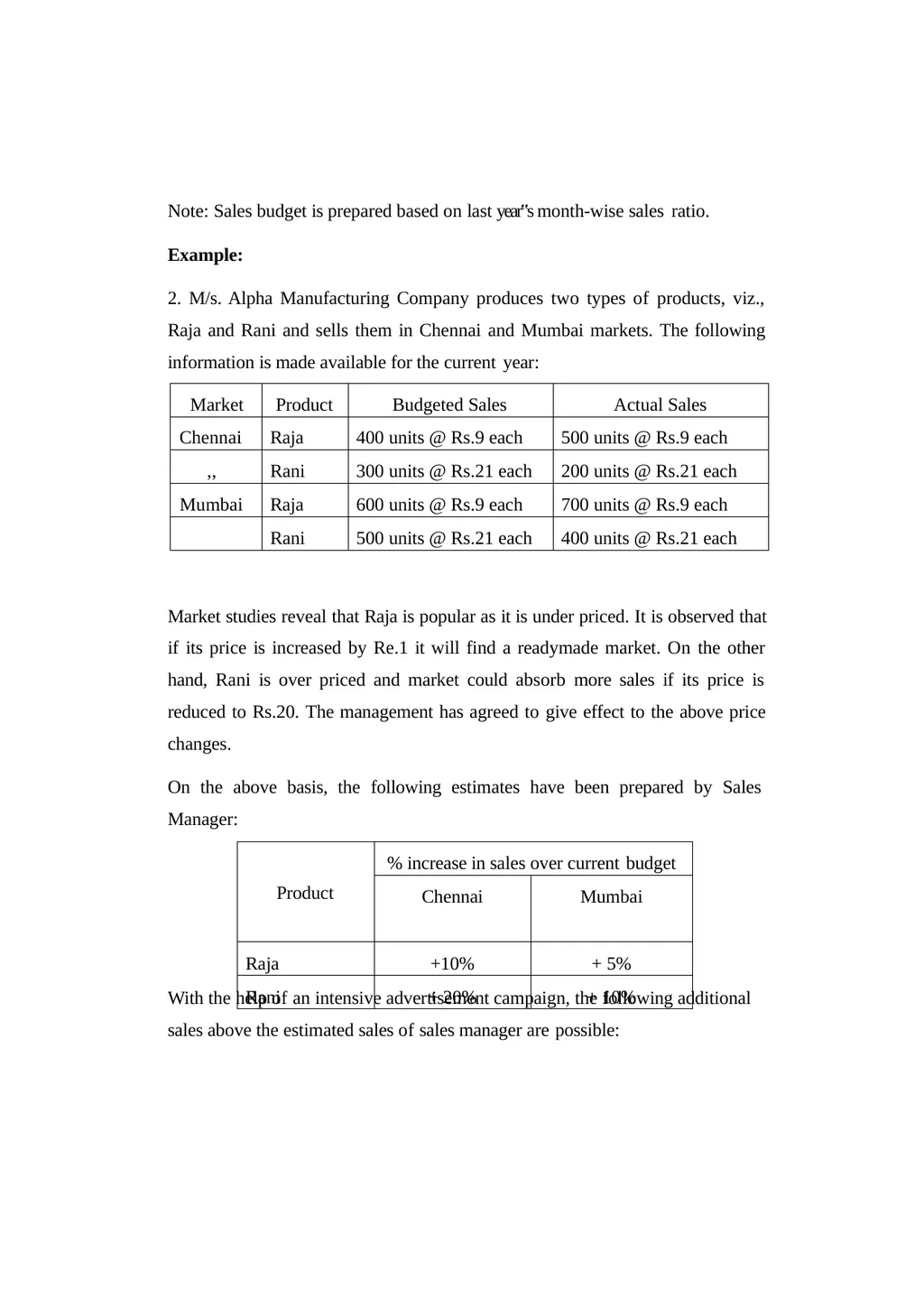
2. M/s. Alpha Manufacturing Company produces two types of products, viz., Raja and Rani and sells them in Chennai and Mumbai markets. The following information is made available for the current year: Market studies reveal that Raja is popular as it is under priced. It is observed that if its price is increased by Re.1 it will find a readymade market. On the other hand, Rani is over priced and market could absorb more sales if its price is reduced to Rs.20. The management has agreed to give effect to the above price changes.
On the above basis, the following estimates have been prepared by Sales Manager: With the help of an intensive advertisement campaign, the following additional sales above the estimated sales of sales manager are possible:<br>
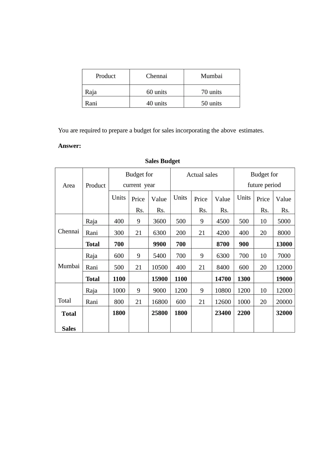
slide42. You are required to prepare a budget for sales incorporating the above estimates.
Answer:
Sales Budget<br>
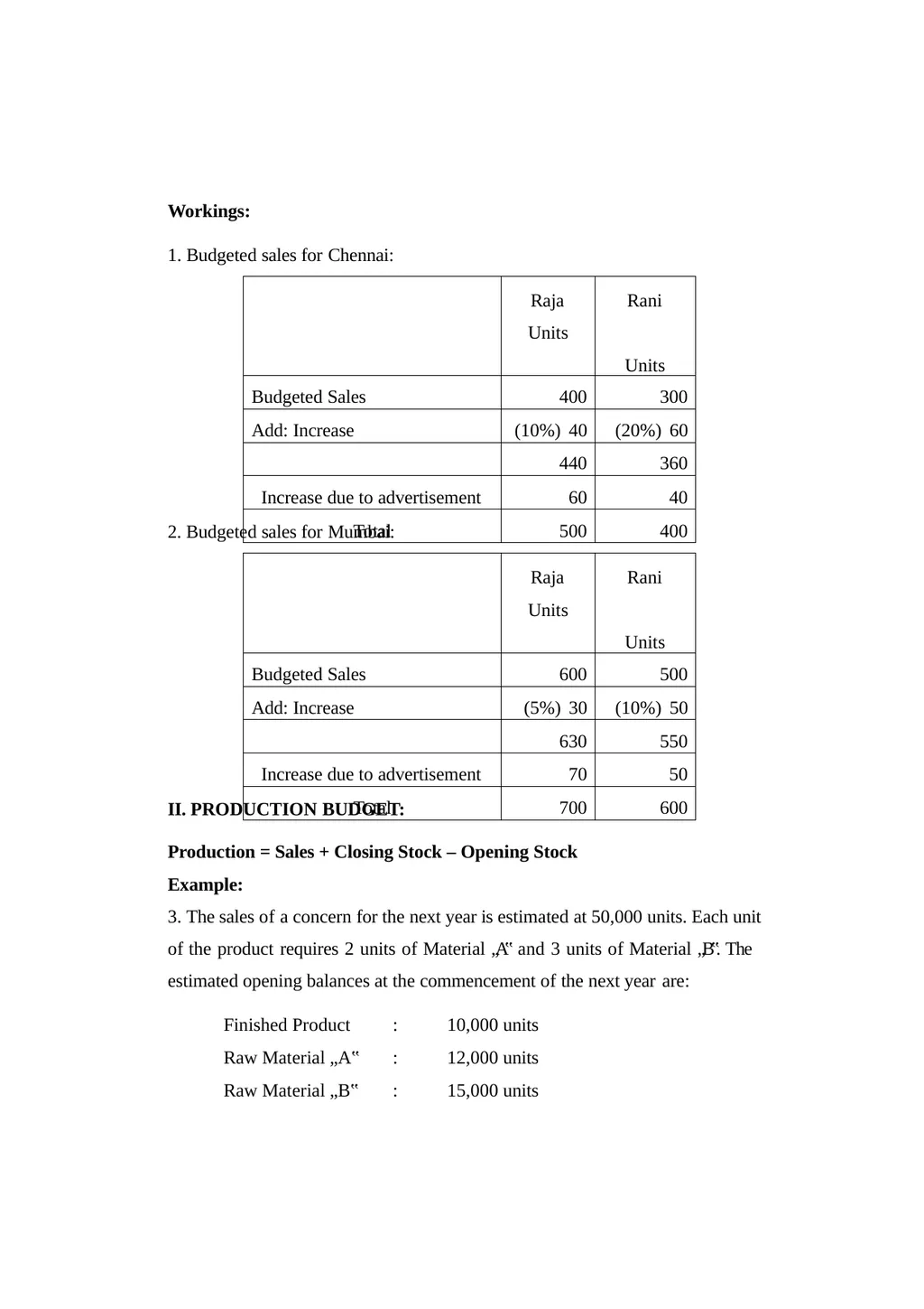
slide43. Workings:
1. Budgeted sales for Chennai: 2. Budgeted sales for Mumbai: II. PRODUCTION BUDGET:
Production = Sales + Closing Stock – Opening Stock Example:
3. The sales of a concern for the next year is estimated at 50,000 units. Each unit of the product requires 2 units of Material „A‟ and 3 units of Material „B‟. The
estimated opening balances at the commencement of the next year are: Finished Product :
Raw Material „A‟ :
Raw Material „B‟ : 10,000 units
12,000 units
15,000 units<br>
slide44. The desirable closing balances at the end of the next year are: Finished Product :
Raw Material „A‟ :
Raw Material „B‟ : 14,000 units
13,000 units
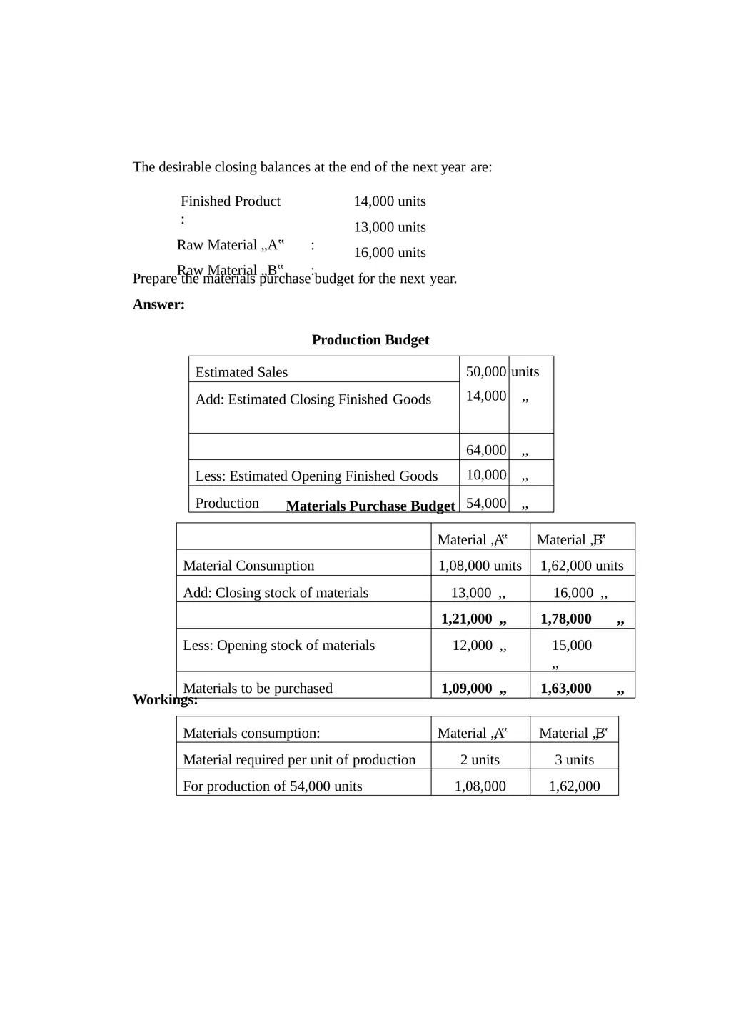
16,000 units Prepare the materials purchase budget for the next year.
Answer:
Production Budget Materials Purchase Budget Workings:<br>
slide45. CASH BUDGET:
It is an estimate of cash receipts and disbursements during a future period of time. “The Cash Budget is an analysis of flow of cash in a business over a future, short or long period of time. It is a forecast of expected cash intake and outlay” (Soleman, Ezra – Handbook of Business administration).
Procedure for preparation of Cash Budget:
First take into account the opening cash balance, if any, for the beginning of the period for which the cash budget is to be prepared.
Then Cash receipts from various sources are estimated. It may be from cash sales, cash collections from debtors/bills receivables, dividends, interest on investments, sale of assets, etc.
The Cash payments for various disbursements are also estimated. It may be for cash purchases, payment to creditors/bills payables, payment to revenue and capital expenditure, creditors for expenses, etc.
The estimated cash receipts are added to the opening cash balance, if any.
The estimated cash payments are deducted from the above proceeds.
The balance, if any, is the closing cash balance of the month concerned.
The closing cash balance is taken as the opening cash balance of the following month.
Then the process is repeatedly performed.<br>
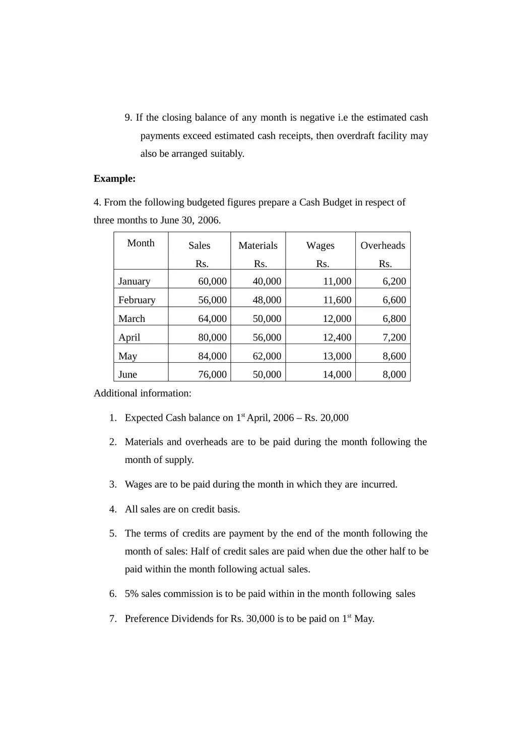
slide46. 9. If the closing balance of any month is negative i.e the estimated cash payments exceed estimated cash receipts, then overdraft facility may also be arranged suitably.
Example:
4. From the following budgeted figures prepare a Cash Budget in respect of three months to June 30, 2006. Additional information:
Expected Cash balance on 1st April, 2006 – Rs. 20,000
Materials and overheads are to be paid during the month following the month of supply.
Wages are to be paid during the month in which they are incurred.
All sales are on credit basis.
The terms of credits are payment by the end of the month following the month of sales: Half of credit sales are paid when due the other half to be paid within the month following actual sales.
5% sales commission is to be paid within in the month following sales
Preference Dividends for Rs. 30,000 is to be paid on 1st May.<br>
slide47. Share call money of Rs. 25,000 is due on 1st April and 1st June.
Plant and machinery worth Rs. 10,000 is to be installed in the month of January and the payment is to be made in the month of June. Answer:
Cash Budget for three months from April to June, 2006<br>
slide48. Workings:
Sales Collection:
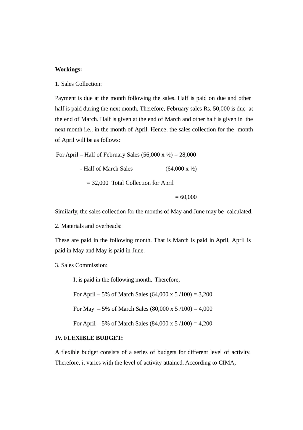
Payment is due at the month following the sales. Half is paid on due and other half is paid during the next month. Therefore, February sales Rs. 50,000 is due at the end of March. Half is given at the end of March and other half is given in the next month i.e., in the month of April. Hence, the sales collection for the month of April will be as follows:
For April – Half of February Sales (56,000 x ½) = 28,000
- Half of March Sales (64,000 x ½) = 32,000 Total Collection for April = 60,000
Similarly, the sales collection for the months of May and June may be calculated.
Materials and overheads:
These are paid in the following month. That is March is paid in April, April is paid in May and May is paid in June.
Sales Commission:
It is paid in the following month. Therefore,
For April – 5% of March Sales (64,000 x 5 /100) = 3,200
For May – 5% of March Sales (80,000 x 5 /100) = 4,000
For April – 5% of March Sales (84,000 x 5 /100) = 4,200
IV. FLEXIBLE BUDGET:
A flexible budget consists of a series of budgets for different level of activity. Therefore, it varies with the level of activity attained. According to CIMA,<br>
slide49. London, A Flexible Budget is, „a budget designed to change in accordance with level of activity attained‟. It is prepared by taking into account the fixed and variable elements of cost. This budget is more suitable when the forecasting of demand is uncertain.
Points to be remembered while preparing a flexible budget:
Cost can be classified into fixed and variable cost.
Total fixed cost remains constant at any level of activity.
Total Variable cost varies in the same proportion at which the level of activity varies.
Fixed and variable portion of Semi-variable cost is to be segregated.
Example:
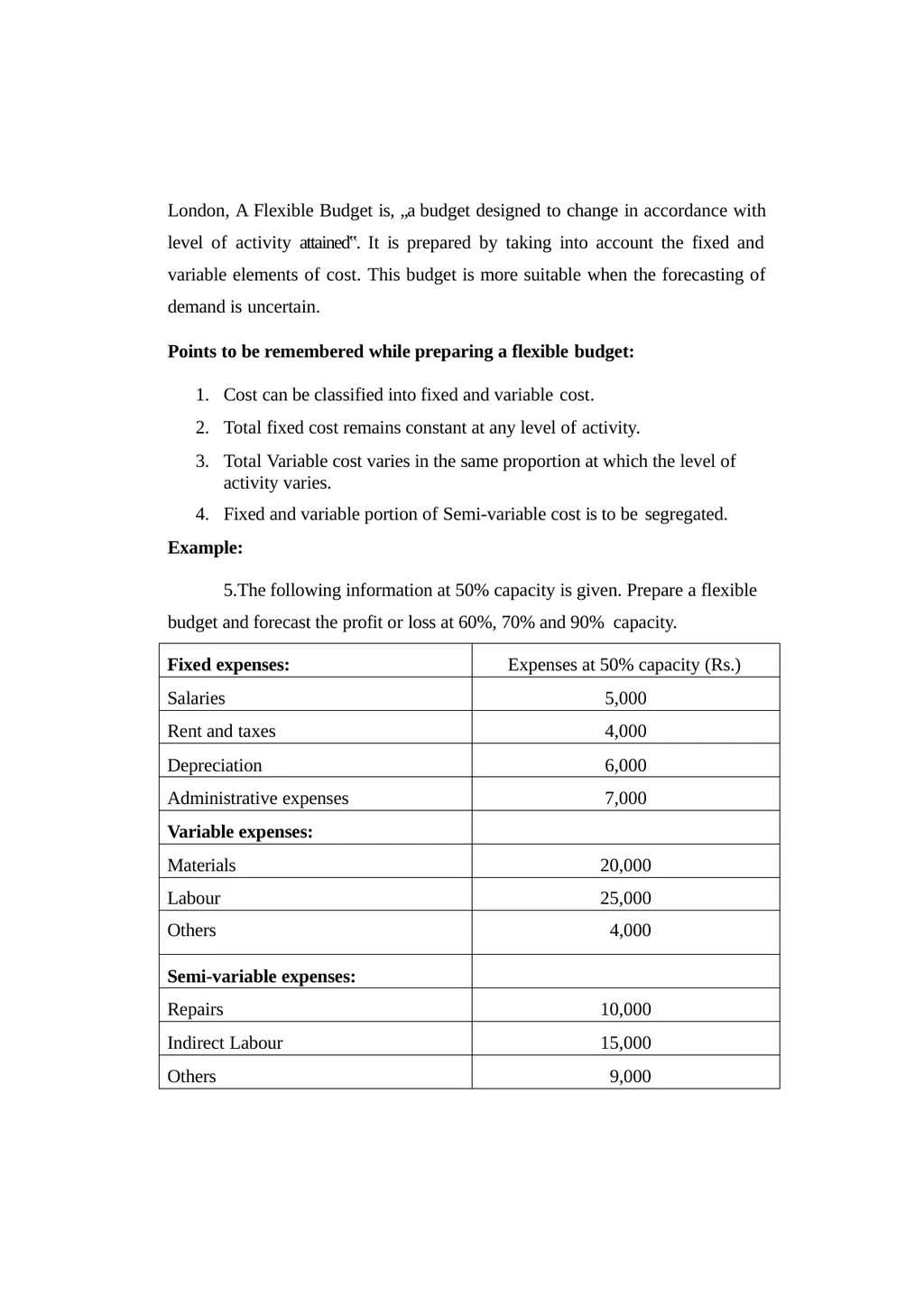
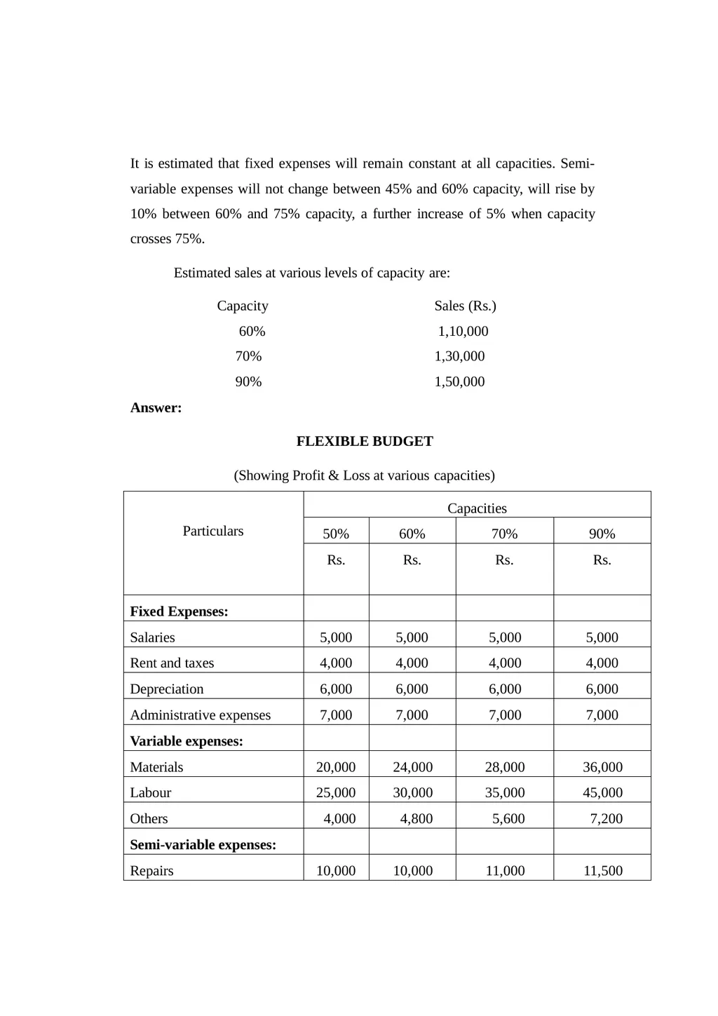
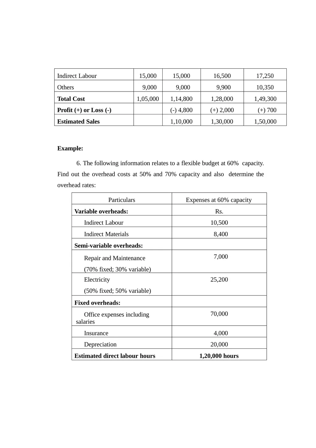
The following information at 50% capacity is given. Prepare a flexible budget and forecast the profit or loss at 60%, 70% and 90% capacity.<br>
slide50. It is estimated that fixed expenses will remain constant at all capacities. Semi- variable expenses will not change between 45% and 60% capacity, will rise by 10% between 60% and 75% capacity, a further increase of 5% when capacity
crosses 75%.
Estimated sales at various levels of capacity are: Capacity 60%
70%
90% Sales (Rs.) 1,10,000
1,30,000
1,50,000 Answer: FLEXIBLE BUDGET
(Showing Profit & Loss at various capacities)<br>
slide51. Example:
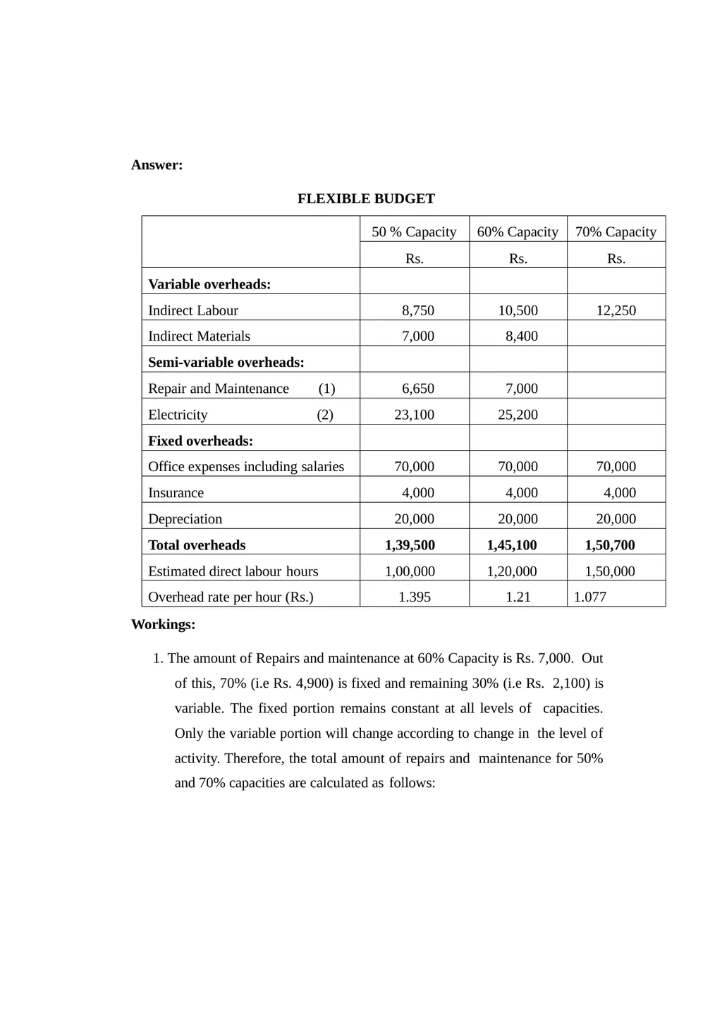
6. The following information relates to a flexible budget at 60% capacity. Find out the overhead costs at 50% and 70% capacity and also determine the overhead rates:<br>
slide52. Answer: FLEXIBLE BUDGET Workings:
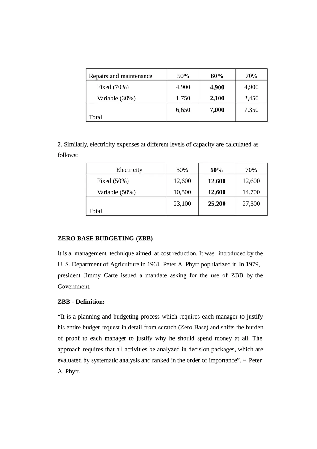
1. The amount of Repairs and maintenance at 60% Capacity is Rs. 7,000. Out of this, 70% (i.e Rs. 4,900) is fixed and remaining 30% (i.e Rs. 2,100) is variable. The fixed portion remains constant at all levels of capacities. Only the variable portion will change according to change in the level of activity. Therefore, the total amount of repairs and maintenance for 50% and 70% capacities are calculated as follows:<br>
slide53. 2. Similarly, electricity expenses at different levels of capacity are calculated as follows: ZERO BASE BUDGETING (ZBB)
It is a management technique aimed at cost reduction. It was introduced by the
U. S. Department of Agriculture in 1961. Peter A. Phyrr popularized it. In 1979, president Jimmy Carte issued a mandate asking for the use of ZBB by the
Government.
ZBB - Definition:
“It is a planning and budgeting process which requires each manager to justify his entire budget request in detail from scratch (Zero Base) and shifts the burden of proof to each manager to justify why he should spend money at all. The approach requires that all activities be analyzed in decision packages, which are evaluated by systematic analysis and ranked in the order of importance”. – Peter
A. Phyrr.<br>
slide54. It implies that-
Every budget starts with a zero base
No previous figure is to be taken as a base for adjustments
Every activity is to be carefully examined afresh
Each budget allocation is to be justified on the basis of anticipated circumstances
Alternatives are to be given due consideration
Advantages of ZBB:
Effective cost control can be achieved
Facilitates careful planning
Management by Objectives becomes a reality
Identifies uneconomical activities
Controls inefficiencies
Scarce resources are used beneficially
Examines each activity thoroughly
Controls wasteful expenditure
Integrates the management functions of planning and control
Reviews activities before allowing funds for them.
PERFORMANCE BUDGETING:
It involves evaluation of the performance of the organization in the context of both specific as well as overall objectives of the organization. It provides a<br>
slide55. definite direction to each employee and a control mechanism to top management.
Definition:
Performance Budgeting technique is the process of analyzing, identifying, simplifying and crystallizing specific performance objectives of a job to be achieved over a period of the job. The technique is characterized by its specific direction towards the business objectives of the organization. – The National Institute of Bank Management.
The responsibility for preparing the performance budget of each department lies on the respective departmental head. It requires preparation of performance reports. This report compares budget and actual data and shows any existing variances. To facilitate the preparation the departmental head is supplied with the copy of the master budget appropriate to his function.
MASTER BUDGET:
Master budget is a comprehensive plan which is prepared from and summarizes the functional budgets. The master budget embraces both operating decisions and financial decisions. When all budgets are ready, they can finally produce budgeted profit and loss account or income statement and budgeted balance sheet. Such results can be projected monthly, quarterly, half-yearly and at year end. When the budgeted profit falls short of target it may be reviewed and all budgets may be reworked to reach the target or to achieve a revised target approved by the budget committee.<br>
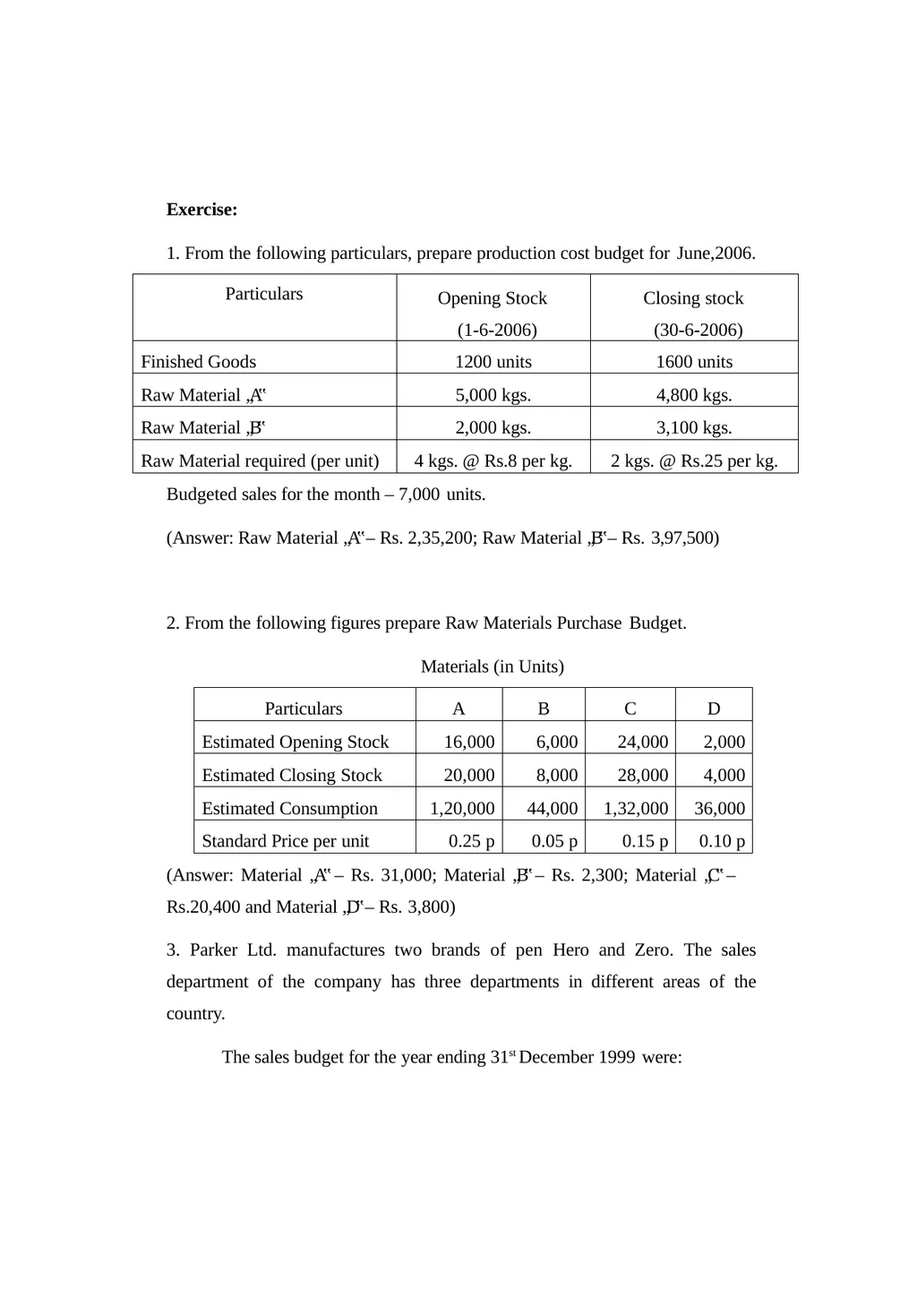
slide56. Exercise:
1. From the following particulars, prepare production cost budget for June,2006. Budgeted sales for the month – 7,000 units.
(Answer: Raw Material „A‟ – Rs. 2,35,200; Raw Material „B‟ – Rs. 3,97,500) 2. From the following figures prepare Raw Materials Purchase Budget.
Materials (in Units) (Answer: Material „A‟ – Rs. 31,000; Material „B‟ – Rs. 2,300; Material „C‟ – Rs.20,400 and Material „D‟ – Rs. 3,800)
3. Parker Ltd. manufactures two brands of pen Hero and Zero. The sales department of the company has three departments in different areas of the country.
The sales budget for the year ending 31st December 1999 were:<br>
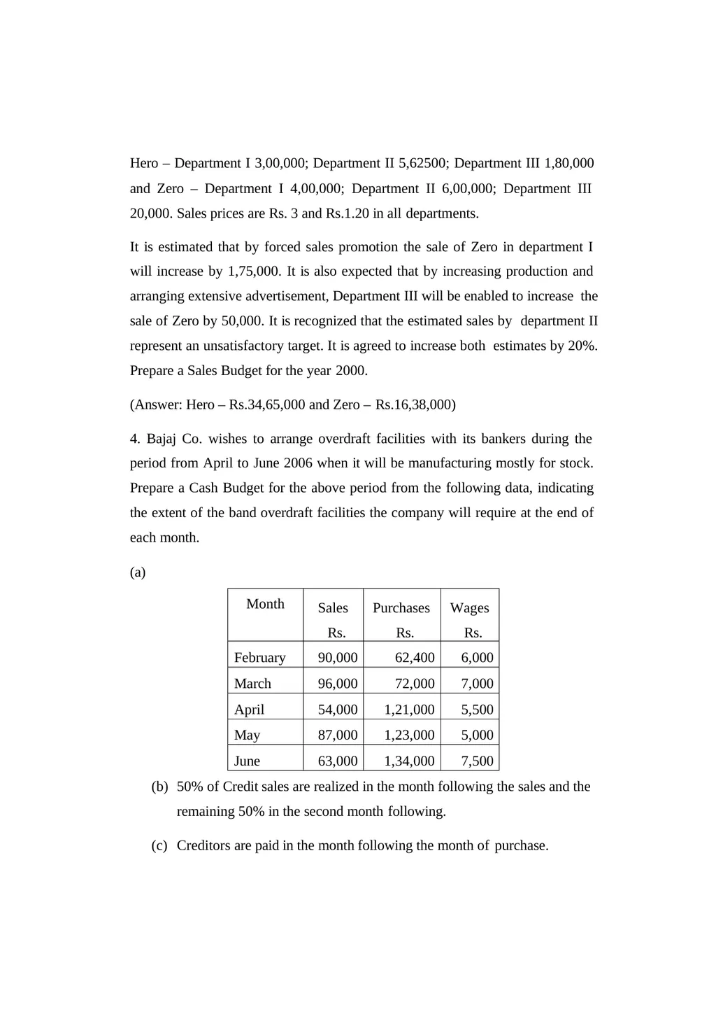
slide57. Hero – Department I 3,00,000; Department II 5,62500; Department III 1,80,000 and Zero – Department I 4,00,000; Department II 6,00,000; Department III 20,000. Sales prices are Rs. 3 and Rs.1.20 in all departments.
It is estimated that by forced sales promotion the sale of Zero in department I will increase by 1,75,000. It is also expected that by increasing production and arranging extensive advertisement, Department III will be enabled to increase the sale of Zero by 50,000. It is recognized that the estimated sales by department II represent an unsatisfactory target. It is agreed to increase both estimates by 20%. Prepare a Sales Budget for the year 2000.
(Answer: Hero – Rs.34,65,000 and Zero – Rs.16,38,000)
4. Bajaj Co. wishes to arrange overdraft facilities with its bankers during the period from April to June 2006 when it will be manufacturing mostly for stock. Prepare a Cash Budget for the above period from the following data, indicating the extent of the band overdraft facilities the company will require at the end of each month.
(a) 50% of Credit sales are realized in the month following the sales and the remaining 50% in the second month following.
Creditors are paid in the month following the month of purchase.<br>
slide58. Lag in payment of wages – one month.
Cash at bank on 1st April, 2006 estimated at Rs. 12,500.
Answer: Closing balance for April – Rs. 26,500; May Rs. (25,500) and June Rs. (83,000)
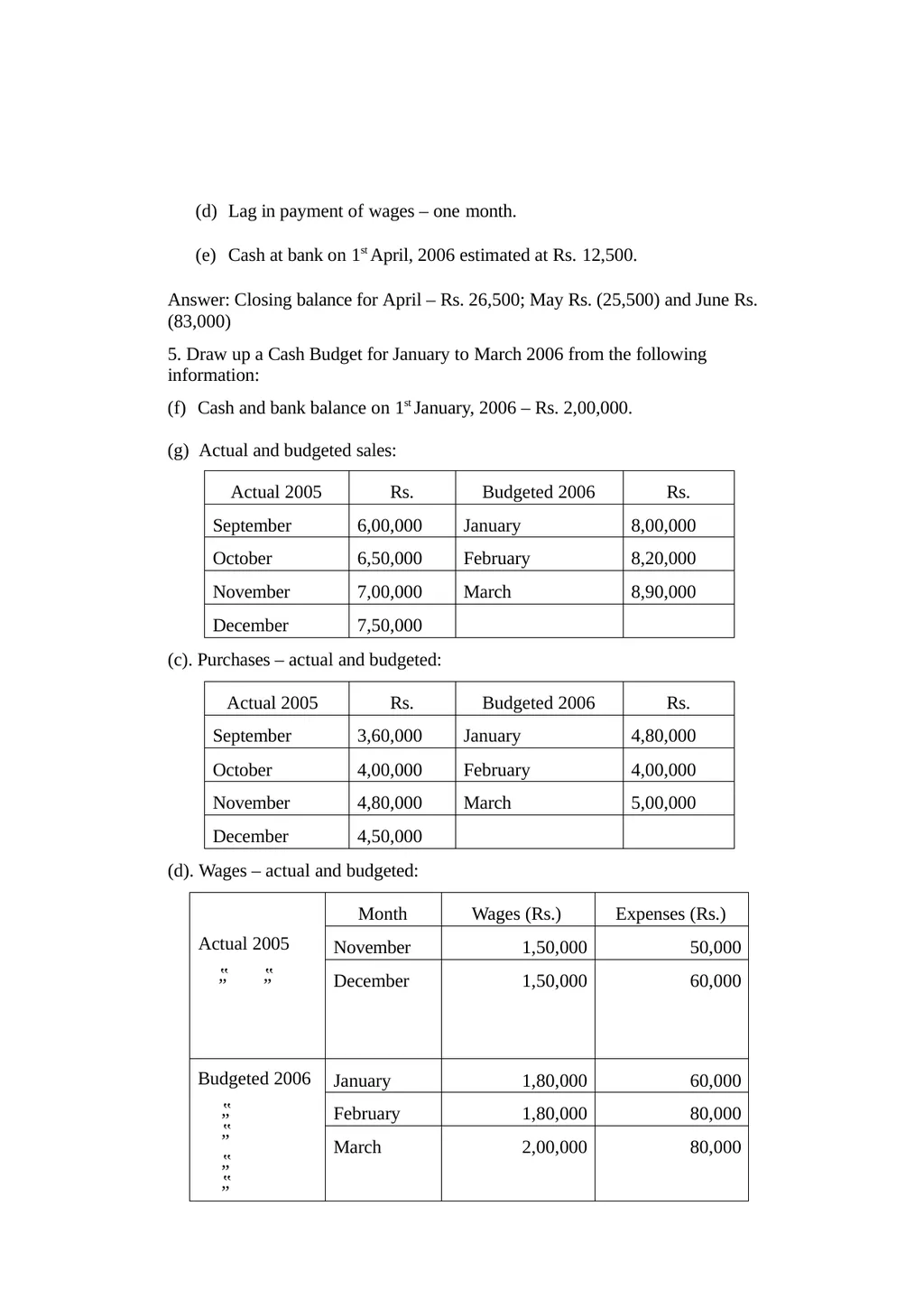
5. Draw up a Cash Budget for January to March 2006 from the following information:
Cash and bank balance on 1st January, 2006 – Rs. 2,00,000.
Actual and budgeted sales: (c). Purchases – actual and budgeted: (d). Wages – actual and budgeted:<br>
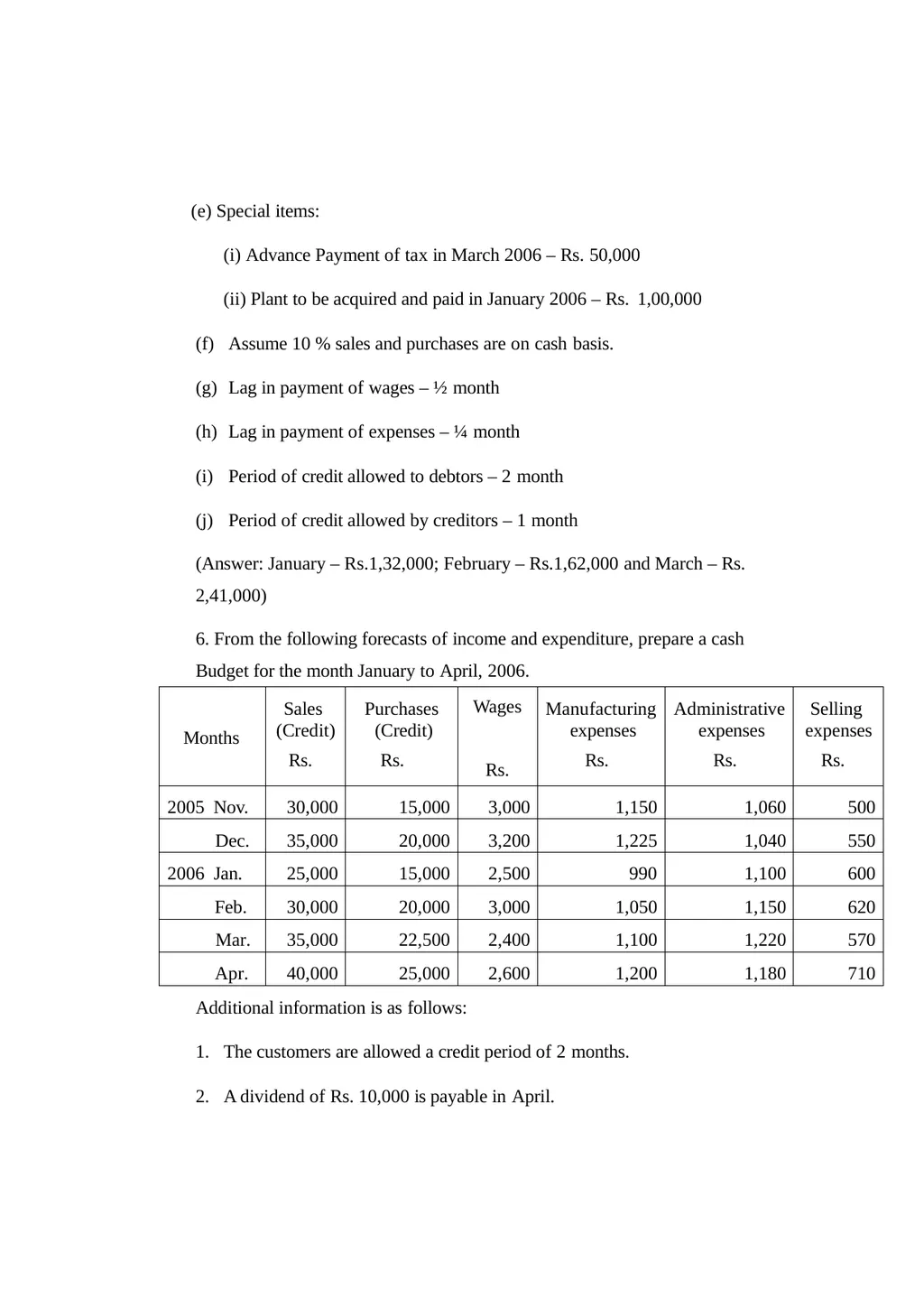
slide59. Special items:
Advance Payment of tax in March 2006 – Rs. 50,000
Plant to be acquired and paid in January 2006 – Rs. 1,00,000
Assume 10 % sales and purchases are on cash basis.
Lag in payment of wages – ½ month
Lag in payment of expenses – ¼ month
Period of credit allowed to debtors – 2 month
Period of credit allowed by creditors – 1 month
(Answer: January – Rs.1,32,000; February – Rs.1,62,000 and March – Rs. 2,41,000)
6. From the following forecasts of income and expenditure, prepare a cash Budget for the month January to April, 2006. Additional information is as follows:
The customers are allowed a credit period of 2 months.
A dividend of Rs. 10,000 is payable in April.<br>
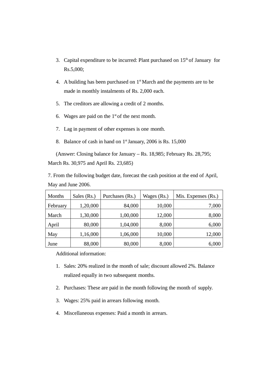
slide60. Capital expenditure to be incurred: Plant purchased on 15th of January for Rs.5,000;
A building has been purchased on 1st March and the payments are to be made in monthly instalments of Rs. 2,000 each.
The creditors are allowing a credit of 2 months.
Wages are paid on the 1st of the next month.
Lag in payment of other expenses is one month.
Balance of cash in hand on 1st January, 2006 is Rs. 15,000
(Answer: Closing balance for January – Rs. 18,985; February Rs. 28,795; March Rs. 30,975 and April Rs. 23,685)
7. From the following budget date, forecast the cash position at the end of April, May and June 2006. Additional information:
Sales: 20% realized in the month of sale; discount allowed 2%. Balance realized equally in two subsequent months.
Purchases: These are paid in the month following the month of supply.
Wages: 25% paid in arrears following month.
Miscellaneous expenses: Paid a month in arrears.<br>
slide61. Rent: Rs.1,000 per month paid quarterly in advance due in April.
Income Tax : First instalment of advance tax Rs. 25,000 due on or before 15th June.
Income from investments: Rs. 5,000 received quarterly in April, July, etc.
Cash in hand: Rs. 5,000 on 1st April, 2006.
(Answer: April – Rs. 5,680; May – Rs. (-) 7,084 and June – Rs. (-) 62,936
8. The Expenses for the production of 5,000 units in a factory are given as follows: You are required to prepare a budget for the production of 7,000 units.
(Answer Total cost of sales Rs. 7,69,000; Total cost of sales per unit Rs. 109.94)
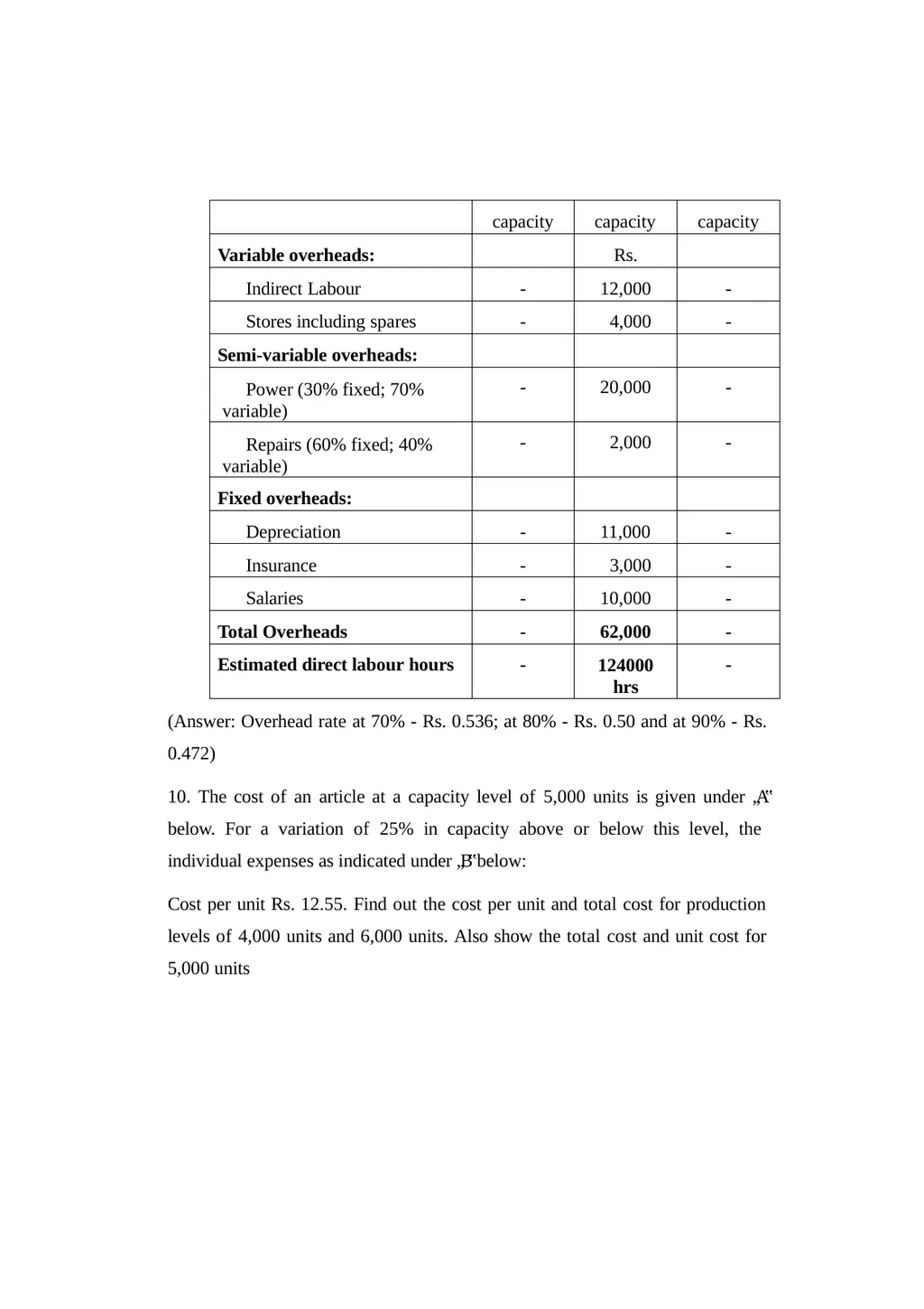
9. Draw up a flexible budget for the overhead expenses on the basis of the following data and determine the overhead rate at 70%, 80% and 90% plant capacity.<br>
slide62. (Answer: Overhead rate at 70% - Rs. 0.536; at 80% - Rs. 0.50 and at 90% - Rs. 0.472)
10. The cost of an article at a capacity level of 5,000 units is given under „A‟ below. For a variation of 25% in capacity above or below this level, the individual expenses as indicated under „B‟ below:
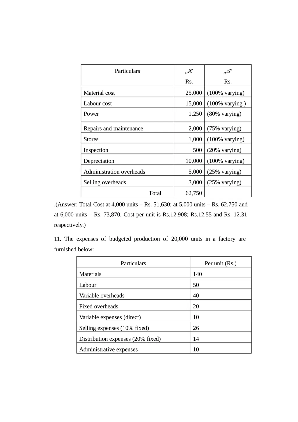
Cost per unit Rs. 12.55. Find out the cost per unit and total cost for production levels of 4,000 units and 6,000 units. Also show the total cost and unit cost for 5,000 units<br>
slide63. .(Answer: Total Cost at 4,000 units – Rs. 51,630; at 5,000 units – Rs. 62,750 and at 6,000 units – Rs. 73,870. Cost per unit is Rs.12.908; Rs.12.55 and Rs. 12.31 respectively.)
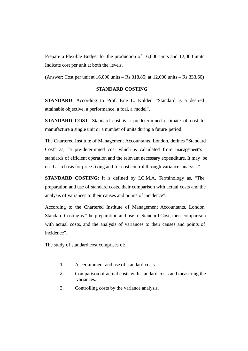
11. The expenses of budgeted production of 20,000 units in a factory are furnished below:<br>
slide64. Prepare a Flexible Budget for the production of 16,000 units and 12,000 units. Indicate cost per unit at both the levels.
(Answer: Cost per unit at 16,000 units – Rs.318.85; at 12,000 units – Rs.333.60)
STANDARD COSTING
STANDARD: According to Prof. Erie L. Kolder, “Standard is a desired attainable objective, a performance, a foal, a model”.
STANDARD COST: Standard cost is a predetermined estimate of cost to manufacture a single unit or a number of units during a future period.
The Chartered Institute of Management Accountants, London, defines “Standard Cost” as, “a pre-determined cost which is calculated from management‟s standards of efficient operation and the relevant necessary expenditure. It may be used as a basis for price fixing and for cost control through variance analysis”.
STANDARD COSTING: It is defined by I.C.M.A. Terminology as, “The preparation and use of standard costs, their comparison with actual costs and the analysis of variances to their causes and points of incidence”.
According to the Chartered Institute of Management Accountants, London Standard Costing is “the preparation and use of Standard Cost, their comparison with actual costs, and the analysis of variances to their causes and points of incidence”.
The study of standard cost comprises of: 1.
2. Ascertainment and use of standard costs.
Comparison of actual costs with standard costs and measuring the variances.
Controlling costs by the variance analysis. 3.<br>
slide65. 4. Reporting to management for taking proper action to maximize the efficiency. BUDGETARY CONTROL AND STANDARD COSTING
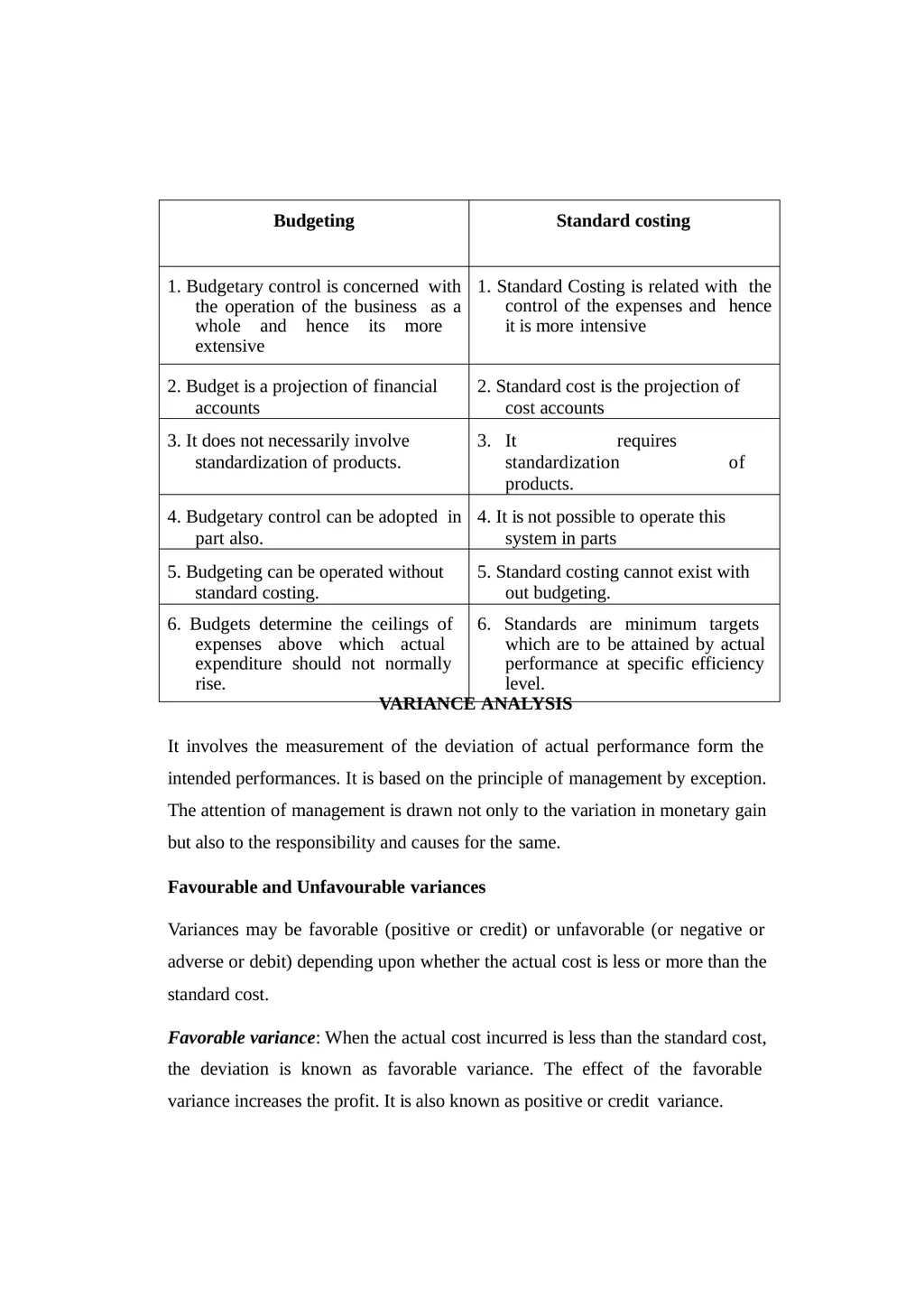
Both standard costing and budgetary control aim at maximum efficiency and managerial control. Budgetary control and standard costing have the common objective of controlling business operations by establishing pre-determined targets, measuring the actual performance and comparing it with the targets, for the purposes of having better efficiency and of reducing costs. The two systems are said to be interrelated but they are not inter-dependent. The budgetary control system can function effectively even without the system of standard costing in operation but the vice-versa is not possible.
STANDARD COSTING AS A CONTROLLING TECHNIQUE
It is essential for management to have knowledge of costs so that decision can be effective. Management can control costs on information being provided to it. The technique of standard costing is used for building a proper budgeting and feedback system. The uses of standard costing to management areas follows.
Formulation of Price and Production Policies
Standard Costing acts as a valuable guide to management in the fixation of price and formulation production polices. It also assists management in the field of inventory pricing, product, product pricing profit planning and also in reporting to higher levels.
Comparison and Analysis of Data
Standard Costing provides a stable basis for comparison of actual with standard costs. It brings out the impact of external factors and internal causes on the cost and performance of the concern. Thus, it helps to take remedial action.<br>
slide66. Cost Consciousness
An atmosphere of cost consciousness is created among the staff. Standard costing also provides incentive to workers for efficient performance.
Better Capacity to anticipate
An effective budget can be formulated for the future by once knowing the deviations of actual costs from standard costs. Data are available at an early stage and the capacity to anticipate about changing conditions is developed.
Better Economy, Efficiency and Productivity
Men, machines and materials are more effectively utilized and thus benefits of economies can be reaped in business together with increased productivity.
Delegation of Authority and Responsibility
The net profit is analyzed and responsibility can be placed on the person in charge for any variations from the standards. It discloses adverse variations and particular cost centre can be held accountable. Thus, delegation of authority can be made by management to control the affairs in different departments.
Management by ‘Exception’
The principle of “management by exception‟ can be applied in the business. This helps the management in concentrating its attention on cases which are off standard, i.e., below or above the standard set. A pattern is provided for the elimination of undesirable factors causing damage to the business.
SETTING THE STANDARD
While setting standard cost for operations, process or products, the following preliminaries must be gone through:<br>
slide67. Establish Standard Committee comprising Purchase Manager, Personnel Manager, and Production Manager. The Cost Accountant coordinates the functions.
Study the existing costing system, cost records and forms in use.
A technical survey of the existing methods of production should be undertaken.
Determine the type of standard to be used.
Fix standard for each element of cost.
Determine standard costs of r each product.
Fix the responsibility for setting standards.
Account variances properly.
Ascertain the deviations by comparing the actual with standards.
Take necessary action to ensure that adverse variances are not repeated.
DETERMINATION OF STANDARD COSTS
The following preliminary steps are considered before setting standards:
Establishment of cost centre
Classification and codification of accounts
Types of standards
Setting the standards.
(a) Establishment of cost centre. For fixing responsibility and defining the lines of authority, cost centre is necessary. “A cost centre is a location, person or item of equipment (or group of these) for which costs may be<br>
slide68. ascertained and used of the purpose of cost control”. With the help of cost centre, the standards are prepared and the variances are analyzed.
Classification and codification of accounts. Accounts are classified according to different items of expenses under suitable heading. Each heading may be given codes and symbols. Coding is useful for speedy collection and analysis.
Types of standards. The different types of standards are given below: (i) Basic standard. It is a fixed and unaltered for an indefinite period for forward planning. According to I.C.M.A London, it is “an underlying standard from which a current standard can be developed”. From this basic standard, changes in current standard and actual standard can be measured. (ii) Current standard. It is a short-term standard, as it is revised at regular intervals. I.C.M.A. London refers to it as “a standard which is established for use over a short period of time and is related to current conditions”. This standard is realistic and helpful to business. It is useful for cost control. (iii) Normal standard. It is an average standard, and is based on normal conditions which prevail over a long period of a trade cycle. I.C.M.A defines it as “the average standard which, it is anticipated, can be attained over a future period of time, preferably long enough to cover one trade-cycle”. It is used for planning and decision making during the period of trade cycle to which it is related. It is very difficult to apply in practice.
Ideal standard. I.C.M.A. defines it as “the standard which can be attained under the most favorable condition possible”. It is fixed and (iv)<br>
slide69. needs a high degree of efficiency, best possible conditions of management and performance. Existing conditions and conditions capable of achievement should be taken into consideration. It is difficult to attain this ideal standard.
(v) Expected standard. It is a practical standard. I.C.M.A defines it as, “the standard which, it is anticipated, can be attained during a future specified budget period”. For setting this standard, due weightage is given for all the expected conditions. It is more realistic than the ideal standard.
(d) Setting the standards. After choosing the standard, the setting of standard is the work of the standard committee. The cost accountant has to supply the necessary cost figures and co-ordinate the activity committee. He must ensure that the setting standards are accurate.
Standards cost is determined for each element of the following costs. (i) Direct Material cost. Standard material cost is equal to the standard quantity multiplied by the standard price. The setting of standard costs for direct materials involves Standard Material Quantity. For each product or part or the process, mechanical calculation or mechanical analysis is made. The allowance for normal wastage or loss must be fixed very carefully. Similarly, where different kinds of materials are used as a mix for a process, a standard material mix is determined to produce the desire quality product.
Standard Material Price. Setting of material standard price is done by the cost accountant and the purchase manager. The current standard is the desirable and effective for fixing the price.<br>
slide70. Normally one year is the period for fixation of standard price. If there are more fluctuations in prices, then revision of standard price is necessary. Before fixing the standard, the following points must be considered:
Prices of materials in stock
Price quoted by suppliers
Trade and cash discounts received
Future prices based upon statistical data
Material price already contracted
Setting standard for Direct Labour. The standard labour cost is equal to the standard time for each operation multiplied by the standard wage rate. Setting of standard cost of direct labour involves: (ii) Fixation of standard time
Fixation of standard rate
Fixation of standard time: Standard time is fixed by time or motion study or past records or test runs or estimates. Labour time is fixed by the work study engineer. While fixing standard time, normal ideal time is allowed for fatigue, normal delays or other contingencies.
Fixation of standard rate. With the help of the personnel manager, the accountant determines the standard rate. Fixation of standard rate is influenced by (i) Union‟s policy (ii) Demand for labour (iii) Policy the be followed. (iv) Method of wage payment.<br>
slide71. (iii) Setting standard for Overhead. Overheads are divided into fixed, variable and semi-variable. Standard overhead rate is determined on the basis of past records and future trend of prices. It is calculated for a unit or for an hour. Standard variable overhead rate=
Standard variable overhead for the budge Period
Budgeted production units or budgeted hours for the budgeted period (or some other base)
Standard fixed overhead rate=
Standard overheads for the budget period
Budgeted production units or budgeted hours for the budgeted period (or some other base)
REVISION OF STANDARDS
Standard cost may be established for an indefinite period. There are no definite rules for the selection for a particular period. If the standards are fixed for a short period, it is expensive and frequent revision of standards will impair the utility and purpose for which standard is set.
At the same, if the standard is set for a longer period, it may not be useful particularly in the days of high inflation and large fluctuations of rates in case of materials and labour.
Standards have to be revised from time to time taking into consideration changing circumstances. The circumstances may change on account of technical innovations, changed market conditions, increase or decrease in plant capacity,<br>
slide72. developing new products or giving up unprofitable production lines. If variations from actual occur in practice, they may be due to controllable or uncontrollable causes. Standards should be revised only on account of those causes which are beyond the control of the management. Changes in product design, supply of labour and material, changes in market conditions for a long period, trade or cyclical variations would impel the management to revise the standards. The objective, while comparing the actual performance with the standard performance and revising standards, is to facilitate better control over costs and improve the overall working and profitability of the organization.
Apart from the above, basic standards are revised in the course of time under the following circumstances, when:
There are permanent changes in the method of production –designs and specifications.
Plant capacity is changed
There is a large variation between the standard and the actual.
BUDGETARY CONTROL AND STANDARD COSTING
The systems of budgetary control and standard costing have the common objective of controlling business operations by establishing pre-determined targets, measuring the actual performance and comparing it with the targets, for the purposes of having better efficiency and of reducing costs. The tow systems are said to be interrelated but they are not inter-dependent. The budgetary control system can function effectively even without the system of standard costing in operation but the vice-versa is not true. Usually, the two are used in conjunction with each other to have most fruitful results. The distinction between the two systems is mainly on account of the field or scope and technique of operation.<br>
slide73. VARIANCE ANALYSIS
It involves the measurement of the deviation of actual performance form the intended performances. It is based on the principle of management by exception. The attention of management is drawn not only to the variation in monetary gain but also to the responsibility and causes for the same.
Favourable and Unfavourable variances
Variances may be favorable (positive or credit) or unfavorable (or negative or adverse or debit) depending upon whether the actual cost is less or more than the standard cost.
Favorable variance: When the actual cost incurred is less than the standard cost, the deviation is known as favorable variance. The effect of the favorable variance increases the profit. It is also known as positive or credit variance.<br>
slide74. Unfavorable variance: When the actual cost incurred is more than the standard cost, the variance is known as unfavorable or adverse variance. It refers to deviation to the loss of the business. It is also known as negative or debit variance.
Controllable and Uncontrollable variance:
Variances may be controllable or uncontrollable, depending upon the controllability of the factors causing variances.
Controllable variance: It refers to a deviation caused by such factors which could be influenced by the executive action. For example, excess usage of materials, excess time taken by a worker, etc. When compared to the standard cost it is controllable as the responsibility can be fixed on the in-charge.
Uncontrollable variance: When variance is due to the factors beyond the control of the concerned person (or department), it is uncontrollable. For example, the wage rate increased on account of strike, government restrictions, change in market price etc. Only revision of standards is required to remove such in future.
Uses
The variance analysis are important tools of cost control and cost reduction and they generate and atmosphere of cost consciousness in the organization.
Comparison of actual with standard cost which reveals the efficiency or inefficiency of performance. The inefficiency or unfavorable variance is analyzed and immediate actions are taken.
It is a tool of cost control and cost reduction
It helps to apply the principle of management by exception.<br>
slide75. It helps the management to maximize the profits by analyzing the variances into controllable and uncontrollable; the controllable variances are further analyzed so as to bring a cost reduction, indirectly more profit.
Future planning and programmes are based on the variance analysis.
Within the organization, a cost consciousness is created along with the team spirit.
Computation of variances
The causes of variance are necessary to find remedial measures; and therefore a detailed study of variance analysis is essential. Variances can be found out with respect to all the elements of cost, i.e., direct material, direct labour and overheads. The following are the common variances, which are calculated by the management. Sub-divisions of variances really give detailed information to the management in order to control the cost.
Material variances
Labour variances
Overhead variances (a) variable (b) fixed
Material variance:
The following are the variances in the case of materials
a) Material Cost Variance (MCV). It is the difference between the standard cost of direct materials specified for the output achieved and the actual cost of direct materials used. The standard cost of materials is computed by multiplying the standard price with the standard quantity for actual output; and the actual cost is computed by multiplying the actual price with the actual quantity. The formula is:<br>
slide76. Material Cost Variance (or) MCV:
(Standard cost of materials - Actual cost of materials used)
(or)
(Standard Quantity for actual output x Standard Price) - (Actual Quantity x Actual Rate) (or)
(SO x SP) - (AQ x AP)
b) Material Price Variance (MPV). Material price variance is that portion of the direct materials cost variance which is the difference between the standard price specified and the actual price paid for the direct materials used. The formula is:
Material Price Variance:
(Actual Quantity consumed x Standard Price) – (Actual Quantity consumed x Actual Price) (or)
Actual Quantity consumed (Standard Price - Actual Price)
(or)
MPV= AQ (SP-AP)
c). Material Usage (Quantity) Variance (MUV). It is the deviation caused by the standards due to the difference in quantity used. It is calculated by multiplying the difference between the standard quantity specified and the actual quantity used by the standard price.
Thus material usage variance is “that portion of the direct materials cost variance which is the difference between the standard quantity specified for the production achieved, whether completed or not, and the actual quantity used, both valued at standard prices”.<br>
slide77. Material Usage or Quantity Variance:
Standard Rate (Standard Quantity - Actual Quantity)
(or)
MUV = SR (SQ-AQ)
d) Material Mix Variance (MMV). When two or more materials are used in the manufacture of a product, the difference between the standard composition and the actual composition of material mix is the material mix variance. The variance arises due to the change in the ratio of material and the standard ratio. The formula is:
Material Mix Variance = Standard Rate (Standard Mix – Actual Mix)
Standard is revised due to the shortage of a particular type of material. The formula is:
MMV = Standard Rate (Revised Standard Quantity - Actual Quantity) Revised Standard Quantity (RSQ) =
Total weight of actual mix
x Standard Quantity Total weight of standard mix
After finding out this revised standard mix it is multiplied by the revised standard cost of standard mix and then the standard cost of actual mix is subtracted form the result.
Example:1
The standard cost of material for manufacturing a unit a particular product is estimated as 16kg of raw materials @ Re. 1 per kg.<br>
slide78. On completion of the unit, it was found that 20kg. of raw material costing Rs.
1.50 per kg. has been consumed. Compute Material Variances.
Answer:
MCV = (SQ x SP) - (AQ x AP) = (16 x Rs.1) - (20 x Rs.1.50)
= Rs.16 - Rs.30
= Rs. 14 (Adverse) MPV = (SP – AP) x AQ = (1 – 1.50) x 20 = Rs. 10 (Adverse) MUV = (SQ – AQ) x SP = (16 – 20) x 1 = Rs. 4 (Adverse) Example:2
Calculate the materials mix variance from the following:<br>
slide79. MMV = SR (SQ-AQ)
Material „A‟: MMV = Rs.12 (90-100)
= Rs 12 x10
= Rs. 120(A) Material „B‟: MMV = Rs. 15 (60-50) = Rs. 15 x 10
= Rs 150 (F) Total MMV = Rs. 120(A) + Rs. 150 (F)
= Rs. 30 (F)
(e) Material Yield Variance: It is that portion of the direct material usage variance which is due to the difference between the standard yield specified and the actual yield obtained. The variance arises due to abnormal contingencies like spoilage, chemical reaction etc. Since the variance is a measure of the waste or loss in the production, it known as material loss or waste variance.
ICMA, LONDON, it is defined as “ the difference between the standard yield of the actual material input and the actual yield, both valued at the standard material cost of the produce”. in case actual yield is more than the standard yield, the material yield variance is favourable and, if the actual yield is less than the standard yield, the variance is unfavourable or adverse.
(i) When actual mix and standard mix are the same, the formula is: MYV = Standard Yield Rate (Standard Yield - Actual Yield) or = Standard Revised Rate (Actual Loss - Standard Loss)<br>
slide80. Here Standard Yield Rate =
Standard cost of standard mix
Net standard output Net standard output = Gross output – Standard loss
When the actual mix and the standard mix differ from each other, the formula is:
Standard Rate =
Standard cost of revised standard mix
Net Standard Output
Material Yield Variance=
Standard Rate (Actual Standard Yield – Revised Standard Yield)
Labour Variances
Labour Variances arise because of (I) Difference in Actual Rates and Standard Rates of Labour and (Ii) The variation in Actual Time taken y workers and the Standard Time allotted to them for performing a job. These are computed on the same pattern as that of Material Variances. For Labour Variances by simply putting the word “Time” in place of “Quantity” in the formula meant for Material Variances. The various Labour Variances can be analysed as follows:
Labour Cost Variance
Labour Rate Variance
Labour Time Or Efficiency Variance
Labour Idle Time Variance
Labour Mix Variance Or Gang Composition Variance<br>
slide81. Labour Cost Variance (LCV)
This variance represents the difference between the Standard Labour Costs and the Actual Labour Costs for the production achieved. If the Standard Cost is higher, the variation is favourable and vice versa. It is calculated as follows:
Labour Cost Variance: = (Standard Cost of Labour - Actual Cost of Labour)
= (Standard Time x Standard Rate) - (Actual Time x Actual Rate)
= (ST x SR) - (AT x AR)
Labour Rate Variance (LRV)
It is the difference between the Standard Rate of pay specified and the Actual Rate Paid. According to ICMA, London, the variance is “the difference between the standard and the actual direct Labour Rate per hour for the total hours worked. If the standard rate is higher, the variance is Favourable and vice versa.
Labour Rate Variance = Actual Time (Standard Wage Rate x Actual Wage Rate) V
=AT (SR-AR)
C) Labour Time Or Labour Efficiency Variance (LEV)
It is the difference between the Standard Hours for the actual production achieved and the hours actually worked, valued at the Standard Labour Rate. When the workers finish the specific job in less than the Standard Time, the variance is Favourable. If the workers take more time than the allotted time, the variance is Adverse.
Labour Efficiency Variance (LEV):
=Standard Rate (Standard Time - Actual Time)<br>
slide82. =SR (ST-AT)
Idle Time Variance: It arises because of the time during which the Labour remains idle due to abnormal reasons, i.e. power failure, strikes, machine breakdown, shortage of materials, etc. It is always an Adverse variance
Labour Idle Time Variance = Actual Idle Time x Standard Hourly Rate
Labour Mix Variance or Gang Compostion Variance (LMV):
It is the difference between the standard composition of workers and the actual gang of workers. It is a part of labour efficiency variance. It corresponds to material mix variance. It enables the management to study the labour cost variance occurred because of the changes in the composition of labour force.
The rates of pay of the different categories of workers-skilled, semi-skilled and unskilled are different. Hence, any change made in composition of the workers will naturally cause variance. How much is variance due to the change, is indicated by Labour Mix Variance.
When the total hours i.e. time of the standard composition and actual composition of workers does not differ the formula is:
Labour Mix variance= (Standard Cost of Standard Mix) - (Standard cost of Actual Mix)
When the total hours i.e. time of the standard composition and actual composition of workers differs, the formula is:
Labour Mix variance
Total Time of Actual mix
……………………………. x Std cost of Std. mix) - (Std. cost of Actual Mix) Total Time of Standard mix<br>
slide83. If, on account of short availability of some category of workers, the standard composition is itself revised, then Labour Mix Variance will be calculated by taking revised standard mix in place of standard mix.
Labour Yield Variance (LYV)
It is just like Material Yield Variance. It is the difference between the standard labour output and actual output of yield. It is calculated as below:
Labour Yield Variance
=Standard cost per unit {Standard production of Actual mix - Actual Production}
OVERHEAD VARIANCE
Overhead Cost Variance
It is the difference between standard overheads for actual output i.e. Recovered Overheads and Actual Overheads. It is the total of both fixed and variable overhead variances. The variable overheads are those costs which tend to vary directly in proportion to changes in the volume of production. Fixed overheads consist of costs which are not subject to change with the change in the volume of production. The variances under overheads are analysed in two heads, viz Variable Overheads and Fixed Overheads:
Overheads Cost Variance= Standard Total Overheads-Actual Total Overheads
The term overhead includes indirect material, indirect labour and indirect expenses and the variances relate to factory, office or selling and distribution overheads. Overhead variances are divided into two broad categories: (i) Variable overhead variances and (ii) Fixed overhead variances. To compute overhead variances, the following terms must be understood:<br>
slide84. Standard overhead rate per unit
Budgeted overheads
= …………………… Budgeted output
Standard overheads rate per hour
Budgeted overheads
= ……………………… Budgeted hours c) Standard hours for actual output
Budgeted hours
……………………. Budgeted output x Actual output Standard output for actual time
Budgeted output
……………………. x Actual hours Budgeted hours
Recovered or Absorbed overheads = Standard rate per unit x Actual output
Budgeted overheads = Standard rate per unit x budgeted output
Standard overheads = Standard rate per unit x Standard output for actual time
Actual overheads = Actual rate per unit x Actual output<br>
slide85. VARIABLE OVERHEAD VARIANCE
Variable cost varies in proportion to the level of output, while the cost is fixed per unit. As such the standard cost per unit of these overheads remains the same irrespective of the level of output attained. As the volume does not affect the variable cost per unit or per hour, the only factors leading to difference is price. It results due to the change in the expenditure incurred.
Variable Overhead Expenditure Variance:
It is the difference between actual variable overhead expenditure incurred and the standard variable overheads set in for a particular period. The formula is:-
{Actual Hours Worked x Standard Variable Overhead Rate per hour}-Actual Variable overheads
Variable Overhead Efficiency Variance:
It shows the effect of change in labour efficiency on variable overheads recovery. The formula is:- Standard Rate (Standard Quantity-Actual Quantity)
Standard Overhead Rate= (Standard Time for Actual output- Actual Time)
Variable Overhead Variance
It is divided into two: Overhead Expenditure Variance and Overhead Efficiency Variance. The formula is:-
Variable overhead Expenditure Variance + Variable overhead Efficiency variance
FIXED OVERHEAD VARIANCE (FOV):
Fixed overhead variance depends on (a) fixed expenses incurred and (b) the volume of production obtained. The volume of production depends upon (i)<br>
slide86. efficiency (ii) the days for which the factory runs in a week (calendar variance)
(iii) capacity of plant for production.
FOV = Actual Output (Fixed Overhead Rate - Actual Fixed Overheads)
Fixed Overhead Expenditure Variance. (Budgeted or cost Variance). It is that portion of the fixed overhead which is incurred during a particular period due to the difference between the budgeted fixed overheads and the actual fixed overheads.
Fixed Overhead expenditure variance=Budgeted fixed overhead-Actual fixed overhead
Fixed Overhead Volume Variance. This variance is the difference between the standard cost of overhead absorbed in actual output and the standard allowance for that output. This variance measures the over of under recovery of fixed overheads due to deviation of actual output form the budgeted output level.
On the basis of units of output:
Fixed Overhead Volume Variance = Standard Rate (Budgeted Output-Actual Output) OR
=Budgeted Cost –Standard Cost)
OR
= (Actual Output x Standard Rate)-Budgeted fixed overheads
On the basis of standard hours: Fixed Overhead Volume Variance
=Standard Rate per hour (Budgeted Hours-Standard Hours) Standard Hour = Actual Output + Standard Output per hour<br>
slide87. Example: 3
A manufacturing concern furnished the following information:
Standard: Material for 70kg, finished products:100kg; Price of materials:Re.1 per kg
Actual: Output: 2,10,000 kg; Material used: 2,80,000; cost of material: Rs.5,52,000.
Calculate:-
(a) Material Usage Variance (b) Material Price Variance (c) Material Cost Variance
Answer:
Standard quantity:
For 70kg standard output
Standard quantity of material = 100 kg 2,10,000 kg of finished products
2,10,000 x 100
= …………………………………….. =3,00,000 kg 70
Actual Price per kg
2,52,000
=……………… = Re. 0.90 2,80,000
(a) Material Usage or Quantity Variance
=SP (SQ-AQ)
=Re.1 (3,00,000-2,80,000)
=Re.1 * 20,000
= Rs.20,000 (Favourable)<br>
slide88. (b) Material Price Variance
= AQ (SP - AP)
=2, 80,000 (Re.1 – Re.0.90)
=2, 80,000 * 0.10 paise
= Rs. 28,000 (Favourable)
Material Cost Variance (MCV):
= (SQ x SP) - (AQ x AP)
= (3, 00,000 x 1) – (2,80,000 x 0.90)
= Rs. 3, 00,000 – Rs.2,52,000
= Rs. 48,000 (Favorable)
Example: 4
Standard mix for production of “X‟
Material A: 60 tonnes @ Rs. 5 per tonne Material B: 40 tonnes @ Rs.10 per tonne
Actual mixture being:
Material A: 80 tonnes @ Rs.4 per tonne Material B: 70 tonnes @ Rs. 8 per tonne.
Calculate
Material Price Variance
Material sub-usage Variance, and
Material Mix Variance<br>
slide89. Answer:
Material Price Variance
= AQ (SP - AP)
Material A= 80 (5-4) = Rs.80 (Favourable) Material B= 70 (10-8) = Rs. 140 (Favourable)
MPV = 80 +140 -= Rs 220 (Favourable)
Revised standard quantity=
Total weight of actual mix
* standard quantity Total weight of standard mix
RSQ for material „A‟
150
= ……… * 60 = 90 tonnes 100
RSQ for material „B‟
150
= ……… * 40 = 60 tonnes 100
Material sub usage (Revised usage) Variance =
Standard Price (Standard. Quantity – Revised Standard Quantity) RUV for material „A‟= 5(60-90) = 150 (Adverse)
RUV for material „B‟ = 10(40-90) = 200(Adverse) MRV = 150+200= Rs. 350 (Adverse)
Material Mix Variance = Standard Rate x (Revised std. Quantity - Actual qty.)<br>
slide90. MVV for material „A‟= 5(90-80) =50 (Adverse)
MVV for material „B‟= 10(60-70) =100 (Adverse) MVV=50-100=-50=Rs.540 (Adverse)
Example: 5
Vinak Ltd. produces an article by blending two basic raw materials. It operates a standard costing system and the following standards have been set for new materials. Material A
B Standard Mix 40%
60% Standard price per kg Rs. 4.00
Rs. 3.00 The standard loss in processing is 15%
During April 1994 the company produced 1700 kgs of finished output. The position of stocks and purchases for the month of April 1994 is as under: Calculate: Material Price Variances, Material Usage Variances, Material yield variances, Material Mix Variances and Total Material Cost Variances.<br>
slide91. Answer:
Finished output 1,700 kgs. Standard Loss in processing 15%.
Therefore, input is
100
1,700 x …….. = 2000kgs
85
For an input of 2,000 kgs., the standard cost will be as follows A - 40% of 2000 = 800 kgs. at Rs. 4.00 = Rs. 3,200
B - 60% of 2,000 =1,200 kgs at Rs.3.00 = Rs. 3,600 6,800
Standard Yield Rate =………= Rs. 4 per kg
1,700
Actual Costs:
A - 35+800-5 = 830kgs. consumed 35 x 4 (assumed) = Rs. 140.00
795 x 4.25 (purchase price) = Rs. 3,378.75
……………. Rs. 3,518.75 B 40+ 1,200-50=1190kgs. consumed 40 x 3 (assumed)= 120.00<br>
slide92. 1150 x 2.50(purchase price) =2,875.00 Material Price Variance = AQ (SP-AP)
A = 830 x 4 = 3,320 - 3,518.75 = Rs.198.75 (A) B = 1,190 x 3=3,570 - 2,995 = Rs. 575.00 (F)
…………….. Rs. 376.25 (F)
……………… Material Usage Variance = SP(SQ-AQ) A = 4 (800-830)
B= 3 (1,200-1,190) =120(A)
=30(F)
………. Rs. 90(A) Material Yield Variance = SYR* (AY-SY)
=4(1,700-1,717)=68(A)
If SY For 2,000 kgs. input SY=1,700 Then, For 2,020 kgs. input SY = ?
2,020
=…………. x 1,700=1,717 kgs } 2,000<br>
slide93. Material Mix Variance = SP (RSQ-AQ)
Revised standard quantity=
Total weight of actual mix
x Standard Quantity Total weight of standard mix 2.020
= 800 x ………… = 808
2,000 For „A‟ 2,020
For „B‟= 1,200 x …………..=1,212
2,000 MMV - For „A‟ = 4 (808-803) For „B‟ = 3 (1,212-1,190) = 88(A)
= 66(F) ….. ……………….
Rs. 22(A)
……………………
Material Cost Variance
= (SC - AC) = (6,800 - 6,513.75) = Rs. 286.25(F)
Labour Variance:
Example: 6
With the help of following information calculate
(a) Labour Cost Variance<br>
slide94. Labour Rate Variance
Labour Efficiency Variance Standard hours: 40@ Rs. 3 per hour Actual hours: 50@ Rs. 4 per hour
Answer:
Labour Cost Variance = (Standard Time x Standard Rate) - (Actual Time x Actual Rate)
= (40 x Rs.3) – (50 x Rs.4)
= (Rs.120 - 200) = Rs.80
= Rs.80 (Adverse)
Labour Rate Variance = Actual Time (Standard Rate x Actual Rate)
= 50 (Rs.3 - Rs.4) = Rs. 50
= Rs. 50 (Adverse)
Labour Efficiency Variance = Standard Rate (Standard Time-Actual Time)
= Rs.3 (40-50) = Rs.30
= Rs.30 (Adverse)
Example; 7
The Labour budget of a company for a week is as follows: 20 skilled men @ 50 paise per hour for 40 hours =400
40 skilled men @ 30 paise per hour for 40 hours =480
…….. 880
…….. The actual labour force was used as follows:
30 skilled men @ 50 paise per hour for 40 hours` 30 skilled men @ 35 paise per hour for 40 hours =600
=420
……. 1,020<br>
slide95. Analyses labour variances.
Answer: 1. Labour Rate Variance
Skilled men
Unskilled men
2. Labour Mix variance
Skilled men
Unskilled men
Total Labour Cost Variance = AT (SR - AR)
= 1,200 (Rs.50 - Rs.50) = 0
= 1,200 (Rs.30 - Rs.35) = Rs.60 (A)
= SR (ST - AT)
= Rs.0.50 (800 -1200) = Rs.200 (A)
= Rs.0.30 (1600 -1200) = Rs.120 (F)
= Standard labour cost - Actual cost
= 880-1020 = 140 (A) Example; 8
Standard labour hours and rate for production of Article A are given
below: Calculate: Labour Cost Variance, Labour Rate Variance, Labour Efficiency Variance and Labour Mix Variance<br>
slide96. Answer:
(a) Labour Cost Variance
= (Standard Time x Standard Rate) - (Actual Time x Actual Rate) Standard Time for Actual Production =Actual Units x ST.
Skilled Worker = 1,000 x 5 = 5000 Hrs.
Unskilled worker = 1,000 x 8 = 8,000 Hrs.
Semi-skilled worker= 1,000 x 4 = 4,000 Hrs.
Labour Cost Variance Skilled worker = (5000 x Rs.1.50) – (4,500 x 2)
= Rs.7,500 – Rs.9,000 = Rs.1,500 (A)
= Rs. (8,000 x Rs.0.50) – (10,000 x 0.45)
= 4,000 - 4,500 = Rs.500 (A)
= (4,000 x Rs.0.75) – (4,200 x Rs.0.75)
= 3,000-3,150) = Rs.150 (A) Unskilled worker Semi skilled worker Total Labour Cost Variance = Rs.2150 (A)
(b) Labour Rate Variance = Actual Time (Standard Rate x Actual Rate) Skilled worker Unskilled worker Semi skilled worker = 4500 (1.50 - 2) = Rs.2250 (A)
= Rs.4,200 (0.75 – 0.75) = Nil
= 1,000 (0.50 - 0.45) = Rs.500 (F) Total Labour Rate Variance = Rs.1,750 (A)
(c) Labour mix variance: = SR (Revised std. Mix of Actual hours worked) – Actual Mix
Revised std. Mix of Actual hours worked
Std Mix
=……………………… x Total Actual Hrs.<br>
slide97. Total Std. Hours
5,000
Skilled worker= …………… x 18,700 = 5,500 Hrs
17,000
8,000
Unskilled worker =………… x 18,700 = 8,800 Hrs.
17,000
4,000
Semi skilled worker =………… x 18,700 = 4,400 Hrs
17,000
Labour Mix Variance: Skilled worker Unskilled worker Semi skilled worker = 1.50 (5,500 - 4,500) = Rs.1,500 (F)
= 0.50 (8,800-10,000) = Rs.600 (A)
= 0.75 (4,400 - 4,200) = Rs.150 (F) Total Labour Mix Variance = Rs.1050 (F)
(d) Labour Efficiency Variance = SR (ST for Actual output – Revised Std. Hrs) Skilled worker Unskilled worker Semi skilled worker = 1.50 (5,000 - 5,500) = Rs.750 (A)
= 0.50 (8,000 - 8,800) = Rs.400 (A)
= 0.75 (4,000 - 4,400) = Rs.300 (A) Total Labour Efficiency Variance = Rs. ,450 (A)<br>
slide98. Overhead Variance:
Example: 9
S.V. Ltd has furnished you the following data: Budgeted fixed overhead rate is Re. 1 per hour. In July 1994, the actual hours worked were 31,500.
Calculate the following variance: (i) Efficiency Variance (ii) Capacity variance
(iii) Volume variance (iv) Expenditure variance and (v) Total overhead variance.
Answer:
Budgeted overhead
Recovered overhead =…………………… x Actual output Budgeted output
30,000
=……….. x 22,000
20,000
= 33,000
(i) Efficiency Variance = Standard Rate per hour (Standard hours for actual production – Actual hours)
= Re. 1 x (33,000 – 31,500)
= Rs.1,500 (F)<br>
slide99. Capacity Variance = Standard Rate per hour x (Actual hours - Budgeted hours)
= Standard overheads - Budgeted overheads
= Re. 1 x (31,500 – 30,000)
= Rs.1500 (F)
Volume variance = Recovered overhead – Budgeted overheads
= Rs. 33,000 – Rs. 30,000
= Rs. 3,000 (F)
Expenditure variance = Budgeted overheads – Actual overheads \ = Rs.30,000 – Rs.31,000
= Rs.1,000 (A) (v) Total overhead variance = Recovered overhead – Actual overheads
= Rs.33,000 – Rs.31,000
= Rs.2,000 (F)
Example: 10
Vinak Ltd.has furnished you the following for the month of August 1994. Calculate the variances.<br>
slide100. Answer:
Standard Overhead Rate per Unit
Budgeted Overheads
=……………………………… Budgeted Output
30,000
…………= 1 hours
30,000
Total standard overhead rate per hour
Budgeted overheads
=……………………..
Budgeted hours
1,05,000
= …………. = Rs.3.50 per hour 30,000
Standard fixed overhead rate per hour
Budgeted fixed overheads
= …………………………..
Budgeted hours
45,000
= ………. = Rs.1.50 30,000<br>
slide101. Standard variable overhead rate per hour
Budgeted variable overheads
=……………………………….
Budgeted hours
60,000
= ……….. = Rs.2 30,000
Overhead cost variance = Recovered overheads – Actual overheads
Recovered overhead = Actual output x Standard Rate per unit
= 32,500 x Rs.3.50 = Rs.1,13,750
Overhead cost variance = 1,13,750 – 1,18,000
= Rs.4,250 (A)
Variable overhead cost variance = Recovered overheads – Actual overheads
= 32,500 hrs x Rs.2 – Rs.68,000
= Rs.3,000 (A)
Fixed overhead cost variance = Recovered overheads – Actual overheads
= 32,500 hrs x Rs.1.50 – Rs.50,000
= 48,750 – 50,000
=Rs.1,250 (A)
Expenditure variance = Budgeted overheads – Actual overheads
= Rs.45,000 – Rs.50,000
= Rs.5000 (A)<br>
slide102. Volume variance = Recovered overheads- Budgeted overheads = 32500 hrs x Rs.1.50 – 45,000
= 48,750 – 45,000
= Rs.3,750 (F)
Efficiency variance = Recovered overheads- standard overheads
OR
Standard rate (Standard hours for actual output – Actual hours)
= 1.50 (32,500 – 33,000)
= Rs.750 (A)
Capacity variance = standard overheads – Budgeted overheads
Or
= Standard Rate (Actual hours - Budgeted hours)
= Rs.1.50 (33,000 – 30,000)
= Rs.4,500 (F)
Calendar variance = Extra / Deficit hours worked x Standard Rate. One extra day has been worked.
.. The Total number of extra hours worked
30,000
= ……….. = 1,200 25
=1,200 x 1.50 = Rs.1,800 (F)<br>
slide103. Note:
(F) – Favourable; (A) – Adverse (or) Unfavaourable
When Standard is more than the Actual, it is favourable variance
When Actual is more than the Standard, it is unfavourable or adverse variance
In place of „Time‟, the term „Hours‟ may also be used.
Disposal of Variances:
Cost variances are disposed of in one of the following ways:
Transfer to profit and loss account, keeping work-in-progress, finished goods and cost of sales at standard cost.
Transfer to cost of sales, thus practically converting the standard cost of sales into actual cost of sales.
Prorating to cost of sales and inventories, either on the basis of units or value, so that both the inventories and cost of goods sold will be shown at actual costs.
Exercises:
1. Following is the data of a manufacturing concern. Calculate:- Material Cost Variance, Material Price Variance and Material usage variance.
The standard quantity of materials required for producing one ton of output is 40 units. The standard price per unit of materials is Rs. 3. During a particular period 90 tons of output was undertaken. The materials required for actual production were 4,000 units. An amount of Rs. 14,000 units. An amount of Rs.14, 000 was spent on purchasing the materials.<br>
slide104. (MCV:Rs.3,200(A), MPV: Rs.2,000 (A), MUV Rs.1,200 (A)
The standard materials required for producing 100 units is 120 kgs. A standard price of 0.50 paise per kg is fixed 2,40,000 units were produced during the period. Actual materials purchased were 3,00,000 kgs. at a cost of Rs. 1,65,000. Calculate Materials Variance. ( MCV - 21,000)
From the data given below, calculate: Material Cost Variance, Material Price Variance and Material Usage Variance (MCV (-) Rs.550 (A), MPV: (-) Rs.1,125 (A), MUV(-) Rs.575 (A)
4 From the following information, calculate material mix variance: (Materials Mix Variance: Rs.50 (A)<br>
slide105. 5 Calculate material mix variance form the data given as such: Due to the shortage of material A, the use of material „A‟ was reduced by 10% and that of „B‟ increased by 5% Ans: (Material Mix Variance = -12 (A)
6. From the following data calculate various material variances: (MCV; Rs.145 (A), MPV: Rs.35 (A), MUV: Rs.110 (A), MMV: Rs.3.3 (F)
7. From the following information, Calculate material yield variance: There is a standard loss of 10%. Actual yield is 125 units. (MYV: Rs.76.3 (A)
8. The standard Mix of a product is as under:<br>
slide106. Ten units of finished product should be obtained from the above mentioned mix.
During the month of January, 1978, ten mixes were completed and the consumption was as follows: The actual output was 90 units. Calculate various material variances.
(MCV: Rs.74 (A), MPV: Rs.26 (A), MUV: Rs.48 (A), MMV: Rs.0.35 (F)
9. Vinak Ltd. produces an articles by blending two basic raw materials. It operates a standard costing system and the following standards have been set for raw materials.<br>
slide107. The standard loss in processing is 15%. During April, 1980, the company produced 1,700 kg of finished output. The position of stock and purchase for the month of April, 1980 are as under: Material Yield Variance and Material Mix Variance.
(MCV: Rs.286 (F), Material Price Variance: Rs. 376.75 Favourable, Material Usage Variance. Rs.90 unfavoruable, Material Mix Variance: Rs. 22 Adverse)
In a manufacturing concern, the standard time fixed for a month is 8,000 hours. A standard wage rate of Rs. 2.25 P. per hour has been fixed. During one month, 50 workers were employed and average working days in a month are 25. A worker works for 7 hours in a day. Total wage bill of the factory for the month amounts to Rs. 21,875. There was a stoppage of work due to power failure (idle time) for 100 hours. Calculate various labour variances.
(LCV: Rs.3875 (A), Rate of pay variance: Rs. 2187.50 (A), LEV: Rs.1462.50 (A)
Idle Time Variance: Rs.225 Adverse.)
The information regarding the composition and the weekly wage rates of labour force engaged on a job scheduled to be completed in 30 weeks are as follows:<br>
slide108. The work was completed in 32 weeks. Calculate various labour variances.
12. The following data is taken out from the books of a manufacturing concern.
Budgeted labour composition for producing 100 articles
20 Men @ Rs. 1.25 hour for 25 hours
30 women @ 1.10 per hour for 30 hours
Actual labour composition for Producing 100 articles
25 Men @ Rs. 1.50 per hour for 24 hours 25 women @ Re. 1.20 per hour for 25 hours
Calculate: (i) Labour Cost Variance, (ii) Labour Rate Variance, (iii) Labour Efficency Variance, (iv) Labour Mix Variance.
Ans:(Labour Cost Variance: Rs. 35 Adverse, Labour Rate Variacne Rs. 212.50 Adverse, LEV:Rs.177.50 Favourable and LMV: Rs.24.38 unfavourable)<br>
slide109. 13. Calculate labour variances from the following data: Ans: LCV Rs.2300 (A), LRV Rs. 1320 (A), LEV Rs 980 (A)
From the following information compute;
Fixed Overhead Variance
Expenditure Variance
Volume Variance
Capacity Variance
Efficiency Variance Budget Actual Ans: Fixed Overhead Variance: Rs. 300 (A), Expenditure Variance: Rs. 400 (A), Volume Variance: Rs. 100 (F), Capacity Variance: Rs. 800 (F), Efficiency Variance: Rs. 700 (A)<br>
slide110. 15. From the following information, calculate various overhead variances: (Total Overhead cost Variance: Rs.14,000 (A), Variable Overhead Variance: Rs. 7,000 (A), Fixed Overhead Variance: Rs.7000 (A),Expenditure Variance: Rs. 13,000 (A), Volume Variance: Rs.6000 (F), Capacity Variance: Rs.1,800 (F), Calendar Variance: Rs.32,780 (F), Efficiency Variance: Rs.420 (F)<br>
slide111. Marginal Costing
Introduction
By analyzing the behaviour of costs in relation to changes in volume of output it becomes evident that there are some items of costs which tend to vary directly with the volume of output, whereas there are others which tend to vary with volume of output, are called variable cost and those remain unaffected by change in volume of output are fixed cost or period costs.
Marginal costing is a study where the effect on profit of changes in the volume and type of output is analysed. It is not a method of cost ascertainment like job costing or contract costing. It is a technique of costing oriented towards managerial decision making and control.
Marginal costing, being a technique can be used in combination with other technique such as budgeting and standard costing. It is helpful in determining the profitability of products, departments, processes, and cost centres. While analyzing the profitability, marginal costing interprets the cost on the basis of nature of cost. The emphasis is on behaviour of costs and their impact on profitability.<br>
slide112. Definition
Marginal costing is defined by the ICWA, India as “the ascertainment of marginal costs and of the effect on profit of changes in volume or type of output by differentiating between fixed costs, and variable costs”
Batty defined Marginal Costing as, “a technique of cost accounting which pays special attention to the behaviour of costs with changes in the volume of output”
Kohler‟s Dictionary for Accounting defines Marginal Costing “as the ascertainment of marginal or variable costs to an activity department or products as compared with absorption costing or direct costing”
The method of charging all the costs to production is called absorption costing. Kohler‟s dictionary for Accountants defines it as “the process of allocating all or a portion of fixed and variable production costs to work – in – process, cost of sales and inventory”. The net profits ascertained under this system will be different from that under marginal costing because of
Difference in stock valuation
Over and under – absorbed overheads
Direct costing is defined as the process of assigning costs as they are incurred to products and services
Features of Marginal Costing
The following are the special features of Marginal Costing:
Marginal costing is a technique of working of costing which is used in conjunction with other methods of costing (Process or job)
Fixed and variable costs are kept separate at every stage. Semi – Variable costs are also separated into fixed and variable.<br>
slide113. As fixed costs are period costs, they are excluded from product cost or cost of production or cost of sales. Only variable costs are considered as the cost of the product.
As fixed cost is period cost, they are charged to profit and loss account during the period in which they incurred. They are not carried forward to the next year‟s income.
Marginal income or marginal contribution is known as the income or profit.
The difference between the contribution and fixed costs is the net profit or loss.
Fixed costs remains constant irrespective of the level of activity.
Sales price and variable cost per unit remains the same.
Cost volume profit relationship is fully employed to reveal the state of profitability at various levels of activity.
Assumptions in Marginal Costing
The technique of marginal costing is based on the following assumptions:
All elements of costs can be divided into fixed and variable.
The selling price per unit remains unchanged at all levels of activity.
Variable cost per unit remains constant irrespective of level of output and fluctuates directly in proportion to changes in the volume of output.
Fixed costs remain unchanged or constant for the entire volume of production.
Volume of product is the only factor which influences the costs.<br>
slide114. Characteristics of Marginal Costing
The essential characteristics and mechanism of marginal costing technique may be summed up as follows:
Segregation of cost into fixed and variable elements: In marginal costing, all costs are segregated into fixed and variable elements.
Marginal cost as product cost: Only marginal (variable) costs are charged to products.
Fixed costs are period costs: Fixed cost are treated as period costs and are charged to costing profit and loss account of the period in which they are incurred.
Valuation of inventory: The work – in – progress and finished stocks are valued at marginal cost only.
Contribution is the difference between sales and marginal cost: The relative profitability of the products or departments is based on a study of “contribution” made by each of the products or departments. Advantages of Marginal Costing
Marginal costing is an important technique of managerial decision making. It is a tool for cost control and profit planning. The following are the advantages of marginal costing technique:
1. Simplicity
The statement propounded under marginal costing can be easily followed as it breaks up the cost as variable and fixed.<br>
slide115. Stock Valuation
Stock valuation cab be easily done and understood as it includes only the variable cost.
Meaningful Reporting
Marginal costing serves as a good basis for reporting to management. The profits are analyzed from the point of view of sales rather than production.
Effect on Fixed Cost
The fixed costs are treated as period costs and are charged to Profit and Loss Account directly. Thus, they have practically no effect on decision making.
Profit Planning
The Cost – Volume Profit relationship is perfectly analysed to reveal efficiency of products, processes, and departments. Break – even Point and Margin of Safety are the two important concepts helpful in profit planning. Cost Control and Cost Reduction
Marginal costing technique is helpful in preparation of flexible budgets as the costs are classified into fixed and variable. The emphasis is laid on variable cost for control. The constant focus is on cost and volume and their effect on profit pave the way for cost reduction.
Pricing Policy
Marginal costing is immensely helpful in determination of selling prices under different situations like recession, depression, introduction of new product, etc. Correct pricing can be developed under the marginal costs technique with the help of the cost information revealed therein.<br>
slide116. 8. Helpful to Management
Marginal costing is helpful to the management in exercising decisions regarding make or buy, exporting, key factor and numerous other aspects of business operations.
Limitations of Marginal Costing
Following are the limitations of marginal costing:
Classification of Cost
Break up of cost into fixed and variable portion is a difficult problem. More over clear cost division of semi – variable or semi – fixed cost is complicated and cannot be accurate.
Not Suitable for External Reporting
Since fixed cost is not included in total cost, full cost is not available to outsiders to judge the efficiency.
Lack of Long – term Perspective
Marginal costing is most suitable for decision making in a short term. It assumes that costs are classified into fixed and variable. In the long term all the cost are variable. Therefore it ignores time element and is not suitable for long term decisions.
Under Valuation of Stock
Under marginal costing only variable costs are considered and the output as well as stock are undervalued and profit is distorted. When there is loss of stock the insurance cover will not meet the total cost.<br>
slide117. Automation
In these days of automation and technical advancement, huge investments are made in heavy machinery which results in heavy amount of fixed costs. Ignoring fixed cost in this context for decision making is irrational.
Production Aspect is Ignored
Marginal costing lays too much emphasis on selling function and as such production aspect has been considered to be less significant. But from the business point of view, both the functions are equally important.
Not Applicable in all Types of Business
In contract type and job order type of businesses, full cost of the job or the contract is to be charged. Therefore it is difficult to apply marginal costing in all these types of businesses.
Misleading Picture
Each product is shown at variable cost alone, thus giving a misleading picture about its cost.
Less Scope for Long – term Policy Decision
Since cost, volume, and profits are interlinked in price determination, which can be changed constantly, development of long term pricing policy is not possible.
Marginal Costing and Absorption Costing
Absorption costing charges all the costs i.e., both the fixed and variable fixed to the products, jobs, processes, and operations. Marginal costing technique charges variable cost. Absorption is not any specific method of costing. It is common name for all the methods where the total cost is charged to the output.<br>
slide118. Absorption Costing is defined by I.C.M.A, England as “the practice of charging all costs, both fixed and variable to operations, processes, or products”
From this definition it is inferred that absorption costing is full costing. The full cost includes prime cost, factory overheads, administration overheads, selling and distribution overheads. Distinction between Absorption Costing and Marginal Costing The difference between marginal costing and absorption costing is shown with the help of the following examples.<br>
slide119. Illustration No: 1 Cost of Production (10000 units)
Per Unit
(Rs. P) 1.50
0.25 Total (Rs) 15000
2500
--------- 17500
--------- Variable cost Fixed Cost Total cost Sales 5000 units at Rs. 2.50 per unit Closing stock 5000 units at Rs. 1.75 Solution: Rs. 125000
Rs. 8750 Under absorption costing, the profit will be calculated as follows:<br>
slide120. Under marginal costing method, the profit will be calculated as follows:
Rs. Closing stock will be valued at Rs.7500 only at marginal cost.
Illustration No: 2
The monthly cost figures for production in a manufacturing company are as under:
Rs. Variable cost Fixed cost 120000
35000 Total cost 155000
Normal monthly sales is Rs. 200000/-. Actual sales figures for the three separate months are:
Ist Month IInd Month IIIrd Month Rs. 200000 Rs. 165000 Rs. 235000<br>
slide121. If marginal cost is not used, stocks would be valued as follows:
Ist Month IInd Month IIIrd Month Opening Stock Rs. 108500 Rs. 108500 Rs. 135625
Closing Stock Rs. 108500 Rs. 135625 Rs. 108500
Prepare two tabulations side by side to summarize these results for each of the three months basing one tabulation on marginal costing theory and the other tabulation along side on absorption cost theory.
Solution:<br>
slide122. Note: Stocks at marginal cost is based on variable portion of the monthly total cost given as follows: 120000
Marginal cost in Rs.108500 = 108500 X -------------
155000 = Rs. 84000 120000
Marginal costs in Rs. 135625 = 135625 X -----------
155000 = Rs. 105000 Differential Costing
The concept of differential cost is a relevant cost concept in those decision situations which involve alternative choices. It is the difference in the total costs of two alternatives. This helps in decision making. It can be determined by subtracting the cost of one alternative from the cost of another alternative. Differential costing is the change in the total cost which results from the adoption of an alternative course of action. The alternative may arise on account of sales, volume, price change in sales mix, etc decisions. Differential cost analysis leads to more correct decisions than more marginal costing analysis. In<br>
slide123. this technique the total costs are considered and not the cost per unit. Differential costs do not form part of the accounting system while marginal costing can be adapted to the routine accounting itself. However, when decisions involve huge amount of money differential cost analysis proves to be useful.
In the illustration given below, differential cost at levels of activity has been shown: Differential cost is generally confused with marginal cost. Of course, these two techniques are similar in some aspects but these also differ in certain other respects.<br>
slide124. Similarities
Both the differential cost analysis and marginal cost analysis are based on the classification of cost into fixed and variable. When fixed costs do not change, both differential and marginal costs are same.
Both are the techniques of cost analysis and presentation and are used by the management in formulating policies and decision making.
Dissimilarities
Marginal cost may be incorporated in the accounting system where as differential cost are worked out for reporting to the management for taking certain decisions.
Entire fixed cost are excluded from costing where as some of the relevant fixed costs may be included in the differential cost analysis.
In marginal costing, contribution and p/v ratio are the main yardstick for evaluating performance and decision making. In differential cost analysis emphasis is made between differential cost and incremental or decremental revenue for making policy decisions.
Differential cost analysis may be used in absorption costing and marginal costing.
Marginal Cost
Marginal cost is the cost of producing one additional unit of output. It is the amount by which total cost increases when one extra unit is produced or the amount of cost which can be avoided by producing one unit less.
The ICMA, England defines marginal cost as, “the amount of any given volume of output by which the aggregate cost are charged if the volume of output is increased or decreased by one unit”.<br>
slide125. In practice, this is measured by the total cost attributable to one unit. In this context, a unit may be single article, a batch of articles, an order, a stage of production, a process etc., often managerial costs, variable costs are used to mean the same.
Features of Marginal Cost
It is usually expressed in terms of one unit.
It is charged to operation, processes, or products.
It is the total of prime cost plus variable overheads of one unit.
Marginal Cost Statement
In marginal costing, a statement of marginal cost and contribution is prepared to ascertain contribution and profit. In this statement, contribution is separately calculated for each of the product or department. These contributions are totaled up to arrive at the total contribution. Fixed cost is deducted from the total contribution to arrive at the profit figure. No attempt is made to apportion fixed cost to various products or departments.
Marginal Cost Equation
For convenience the element of cost statement can be written in the form of an equation as given below:
Sales – Variable Cost = Fixed Cost plus or minus Profit or Loss. Or
Sales – Variable Cost = Fixed Cost plus or minus Profit or Loss
In order to make profit, contribution must be more than fixed cost and to avoid loss, contribution should be equal to fixed cost.
The above equation can be illustrated in the form of a statement.<br>
slide126. Marginal Cost Statement Rs. Sales
Less: Variable Cost xxxxx (xxxx)
------------
xxxxx (xxxx)
-------------
xxxx
------------ Contribution Less: Fixed Cost Profit / Loss Illustration No.3:
A company is manufacturing three products X, Y and Z. It supplies you the following information:
Products
-------------------------------------------- Total fixed overheads Rs. 3000/-<br>
slide127. Prepare a marginal cost statement and determine profit and loss. Solution: Marginal Cost Statement Products ------------------------------------------------------------ Marginal Contribution (A – B)
Less:FixedCost 2500 2000 1000 5500
3000 NetProfit 2500 Contribution:
Contribution is the difference between selling price and variable cost of one unit. The greater contribution from the selling unit indicates that the variable cost is less compared to selling price. Total contribution is the number of units<br>
slide128. multiplied by contribution per unit. Contribution will be equal to the total fixed costs at break even point where profit is zero.
Illustration No.4:
Calculate contribution and profit from the following details: Sales Rs. 12000
Variable Cost Rs. 7000
Fixed Cost Rs. 4000 Solution:
Contribution = Sales – Variable cost
Contribution = Rs. 12000 – Rs. 7000 = Rs. 5000
Profit = Contribution – Fixed Cost
Profit = Rs. 5000 – Rs. 4000 = Rs. 1000
Profit / Volume Ratio
This is the ratio of contribution to sales. It is an important ratio analysing the relationship between sales and contribution. A high p/v ratio indicates high profitability and low p/v ratio indicates low profitability. This ratio helps in comparison of profitability of various products. Since high p/v ratio indicates high profits, the objective of every organisation should be to improve or increase the p/v ratio.<br>
slide129. P / V Ratio = Contribution / Sales x 100 or C / S x 100 (Or)
Fixed Cost + Profit
Sales (Or)
Sales – Variable Cost
Sales
When profits and sales for two consecutive periods are given, the following formula can be applied: Change in Profit
Change in Sales
P / V ratio is also used in making the following type of calculations:
Calculation of Break even point.
Calculation of profit at a given level of sales.
Calculation of the volume of sales required to earn a given profit.
Calculation of profit when margin of safety (discussed below) is given.
Calculation of the volume of sales required to maintain the present level of profit if selling price is reduced.
Margin of safety:
The excess of actual or budgeted sales over the break-even sales is known as the margin of safety.
Margin of safety = actual sales - break-even sales<br>
slide130. So this shows the sales volume which gives profit. Larger the margin of safety greater is the profit. Budget sales - break-even sales
----------------------------
Budget sales Margin of safety ratio = (Or)
Profit P/V Ratio
When margin of safety is not satisfactory, the following steps may be taken into account: a)
b)
c)
d)
e)
P/V ratio. Increase the volume of sales. Increase the selling price.
Reduce fixed cost. Reduce variable cost.
Improve sales mix by increasing the sale of products with The effect of a price reduction will always reduce the P / V ratio, raise the break
– even point shorten the margin of safety.
Angle of incidence:
This is obtained from the graphical representation of sales and cost. When sales and output in units are plotted against cost and revenue the angle formed between the total sales line and the total cost line at the break-even point is called the angle of incidence.<br>
slide131. Large angle indicates a high rate of profit while a narrow angle would show a relatively low rate of profit.
Profit goal:
To earn a desired amount of profit i.e., a profit goal can be reached by the formula given below
Fixed cost + Desired profitability Sales volume to reach profit goal = --------------------------------
Contribution ratio
If the profit goal is stated in terms of profit after taxes Fixed cost + {(desired after-tax
--------------------------------
Contribution ratio profit)/1-tax rate}
Sales volume to reach profit goal = Operating leverage: An important concept in context of the CVP analysis is the operating leverage. This refers to the use of the fixed costs in the operation of a firm, and it accentuates fluctuations in the firm's operating profit due to change in sales. Thus the degree of operating leverage may be defined as the percentage change in operating profit (earning before interest and tax) on account of a change in sales.<br>
slide132. % Change in operating profit
--------------------------------------
% Change in sales (Or) Degree of Leverage DOL= Change in EBIT EBIT
--------------------------------------
Change in sales Degree of Leverage DOL=<br>
slide133. Problems
The selling price of a particular product is Rs.100 and the marginal cost is Rs.65. During the month of April, 800 units produced of which 500 were sold. There was no opening at the commencement of the month. Fixed costs amounted to Rs. 18000. Provide a statement using a) Marginal costing and b) Absorption costing, showing the closing stock valuation and the profit earned under each principle.
From the following information, calculate the amount of contribution and profit.
Rs. 3. Determine the amount of fixed cost from the following.
Rs. 4. Determine the amount of variable cost from the following.
Rs.<br>
slide134. Break Even Analysis
Introduction
Break-even analysis is the form of Cost Volume Profit (CVP) analysis. It indicates the level of sales at which revenues equal costs. This equilibrium point is called the break even point. It is the level of activity where total revenue equals total cost. It is alternatively called as CVP analysis also. But it is said that the study up to the state of equilibrium is called as break even analysis and beyond that point we term it as CVP analysis.
Cost – Volume Profit analysis helps the management in profit planning. Profits are affected by several internal and external factors which influence sales revenues and costs.
The objectives of cost-volume profit analysis are:
To forecast profits accurately.
To help to set up flexible budgets.
To help in performance evaluation for purposes of control.
To formulate proper pricing policy.
To know the overheads to be charged to production at various levels.
Volume or activity can be expressed in any one of the following ways:
Sales capacity expressed as a percentage of maximum sales.
Sales value in terms of money.
Units sold.
Production capacity expressed in percentages.<br>
slide135. Value of cost of production.
Direct labour hours.
Direct labour value.
Machine hours.
The factors which are usually involved in this analysis are:
Selling price
Sales volume
Sales mix
Variable cost per unit
Total fixed cost Break Even Chart
These depict the interplay of three elements viz., cost, volume, and profits. The charts are graphs which at a glance provide information of fixed costs, variable costs, production / sales achieved profits etc., and also the trends in each one of them. The conventional graph is as follows:
This is a simple break even chart. The procedure for drawing the chart is as follows:<br>
slide136. Depict the X - axis as the volume of sales or capacity or production.
Depict the Y – axis as the costs or revenue.
Having known the „0‟ level of activity the same fixed cost is incurred, the fixed cost line is depicted as being parallel to the X – axis.
At „0‟ level of activity, the total cost is equal to fixed cost. Therefore the total cost line starts from the point where the fixed cost line meets the Y – axis.
Next plot the sales line starting from „0 ‟.
The meeting point of the sales and the total cost line is the Break Even Point.
It is also called Break Even Point because at that point there is no profit and loss either.
The costs are just recovery by sales. If a perpendicular line is drawn to the X- axis from the BEP, the meeting point of the perpendicular and X- axis will show the break even volume in units. If a perpendicular line is drawn to meet the Y- axis from the BEP, the meeting point shows the break even volume in money terms.
Other details shown in the break even charts are:
Angle of Incidence
This is the angle of intersection between the sales line and the total cost line. The larger the angle the greater is the profit or loss, as the case may be.<br>
slide137. Margin of Safety
This is the difference between the actual sales level and the break even sales. It represents the “cushion” for the company. The larger the distance between the break even sales volume and the actual sales volume, the company can afford to allow the fall in sales without the danger of incurring losses. If the margin of safety is low i.e., if the distance between the actual sales line and the break even sales line is too short, even a small fall in the sales volume will drive the company into the loss area.
The position of break even point should be ideally closer to the y – axis. This will mean that even a small increase in sales will immediately make the company break even. I t should be noted that beyond the break even point all contribution (Sales – Marginal Cost) will directly increase the profits.
Profit Volume Graph
Profit volume graph is a pictorial representation of the profit volume relationship. It shows profit and loss account at different volumes of sales. It is simplified form of break even chart as it clearly represents the relationship of profit to volume of sales. It is possible to construct a profit volume graph for any data relating to a business firm where a break even chart can be drawn. A profit volume graph may be preferred to a break even chart as profit or losses can be directly read at different levels of activity.
The construction of profit volume graph involves the following steps:
Scale of sale is selected on horizontal axis and that for profit or loss are selected on vertical axis. The area below the horizontal axis is the loss area and that above it is the profit area.
Points of profits of corresponding sales are plotted and joined. The resultant line is profit / loss line<br>
slide138. Illustration No. 1
Draw up a profit – volume of the following: Sales Variable cost Fixed cost Profit Rs. 4 Lakhs
Rs. 2 Lakhs
Rs. 1 Lakhs
Rs. 1 Lakhs Solution The calculation of BEP is based on some assumptions. They are as follows:
The costs are classified as fixed and variable costs.
The variable costs vary with volume and the fixed costs remain constant. 3.The selling price remains constant in spite of the change in volume.
4.The productivity per employee also remains unchanged.
Break-even point can be calculated in terms of units or in terms of rupees.<br>
slide139. Break-Even Point (in Rupees) = Break-Even Point (in Rupees) = Fixed Costs
-------------
P/V Ratio (OR)
Fixed Costs
------------- ---------- Marginal cost per unit/1- Selling price per unit Fixed Costs Break-Even Point (in units) = ------------------------
Contribution per unit Where contribution is sales - variable cost and P/V Ratio is Contribution divided by sales.
Cost-volume-profit relationship with the help of an example
The relationship between cost volume and profit are well defined in CVP analysis. With the given example we can elaborately see the relationship
AB Company is a single product manufacturer whose selling price is Rs. 20 per unit and the variable cost is Rs. 12 per unit. The annual fixed cost is Rs. 160000. The number of units produced and sold is 20000. Now if we analyse the CVP relationship
The contribution per unit is = Selling price -variable cost
= 20 - 12 = Rs.8/-
The total contribution for 20000 units is = 8 x 20000 = 160000
Since the profit = total contribution - fixed cost, we get nil profit. 160000- 160000=0<br>
slide140. This is the break even point where the total cost is equal to the total revenue and the company has no profit and no loss.
Let us see a few alternatives
If the fixed cost is Rs. 120000, then the company may earn a profit of Rs. (160000-120000) = 40000. If the fixed cost is Rs.200000, then it may end in a loss of Rs (200000-160000) = 40000
If the variable cost per unit is increased, say to Rs. 15 in the existing condition, then the contribution will come to Rs (20000 x (20-15) = 100000 and that will result in a loss of Rs. 160000-100000 =40000. If the variable cost per unit is decreased say to Rs.10 then the contribution will come to Rs.20000x (20-10) = 200000. Then the profit will be 200000-160000=40000
The above proves that the variation in the costs varies the profitability of the firm.
If the cost decreases, profit increases and vice versa.
Now we can see how the change in volume alters the profitability. If the sales volume is 10000 instead of 20000 as above and the all the other conditions being the same, the result will be (10000x8) - 160000 = 80000 loss. Likewise if the volume is increased to 30000 it will result in a profit of Rs 30000x8 - 160000 = 80000. This shows that the profit increases with the increase in volume when other conditions are unchanged.
Basic Assumptions of Cost – Volume Profit Analysis
Cost volume profit (C-V-P) analysis, popularly referred to as breakeven analysis, helps in answering questions like: How do costs behave in relation to volume? At what sales volume would the firm breakeven? How sensitive is profit to variations in output? What would be the effect of a projected sales<br>
slide141. volume on profit? How much should the firm produce and sell in order to reach a target profit level?
A simple tool for profit planning and analysis, cost-volume-profit analysis is based on several assumptions. Effective use of this analysis calls for an understanding of the significance of these assumptions which are discussed below:
The behaviour of costs is predictable. The conventional cost-volume-profit model is based on the assumption that the cost of the firm is divisible into two components; fixed costs vary variable costs. Fixed costs remain unchanged for all ranges of output; variable costs vary proportionately to volume. Hence the behaviour of costs is predictable. For practical purposes, however, it is not necessary for these assumptions to be valid over the entire range of volume. If they are valid over the range of output within which the firm is most likely to operate – referred to as the relevant range – cost volume profit analysis is a useful tool.
The unit selling price is constant. This implies that the total revenue of the firm is a linear function of output. For firms which have a strong market for their products, this assumption is quite valid. For other firms, however, it may not be so. Price reduction might be necessary to achieve a higher level of sales. On the whole, however, this is a reasonable assumption and not unrealistic enough to impair the validity of the cost-volume- profit model, particularly in the relevant range of output.
The firm manufactures a stable product – mix. In the case of a multi-product firm, the cost volume profit model assumes that the product – mix of the firm remains stable. Without this premise it is not possible to define the average variable profit ratio when different products have different variable profit ratios. While it is necessary to make this assumption, it must be borne in mind that the<br>
slide142. actual mix of products may differ from the planned one. Where this discrepancy is likely to be significant, cost-volume-profit model has limited applicability.
Inventory changes are nil. A final assumption underlying the conventional cost- volume-profit model is that the volume of sales is equal to the volume of production during an accounting period. Put differently, inventory changes are assumed to be nil. This is required because in cost-volume-profit analysis we match total costs and total revenues for a particular period.
Uses and limitations of Break even analysis Uses of BE analysis are as follows:
1.It is a simple device and easy to understand. 2.It is of utmost use in profit planning.
It provides the basic information for further profit improvement studies.
It is useful in decision making and it helps in considering the risk implications of alternative actions.
It helps in finding out the effect of changes in the price, volume, or cost.
It helps in make or buy decisions also and helpful in the critical circumstances to find out the minimum profitability the firm can maintain.
The limitations of BE analysis is:
The basis assumptions are at times base less. For example, we can say that the fixed costs cannot remain unchanged all the time. And the constant selling price and unit variable cost concept are also not acceptable.
It is difficult to segregate the cost components as fixed and variable costs. 3.It is difficult to apply for multinational companies.<br>
slide143. It is a short-run concept and has a limited use in long range planning.
It is a static tool since it gives the relationship between cost, volume and profit at a given point of time and
It fails to predict future revenues and costs.
Despite the limitation it is remains an important tool in profit planning due to the simplicity in calculation.<br>
slide144. Profit = Contribution – Fixed cost
= Rs.24000 – Rs.15000 = Rs.9000
Illustration No. 3
From the following data, calculate the break-even point of sales in rupees: Selling price Rs.20
Variable cost per unit:
Manufacturing Rs.10 Selling Rs.5 Overhead (fixed):
Factory overheads Rs.500000 Selling overheads Rs.200000 Solution:
Selling price per unit: Rs. 20
Variable Cost per unit: Manufacturing: Selling: Rs. 10
Rs.5 Rs.15 Contribution per unit Rs. 5 Contribution ratio = Rs.5 / Rs.20 =25%
Fixed overheads Factory- Rs.500000
Selling- Rs.200000<br>
slide145. Rs.700000
Break even sales in rupees = Fixed overheads /Contribution ratio
= Rs.700000/25%
= Rs.2800000
Break even sales in units = FC/Contribution per unit
= Rs. 700000/Rs.5
= 140000 units
Illustration No. 4
The following data have been obtained from the records of a company Calculate the break-even point.
Solution:
Changes in profit P/V Ratio = x 100 Changes in sales
= 14000 – 10000
X 100 = 40%
90000- 80000<br>
slide146. Contribution = Sales x P/V Ratio = 90000 x 40% = Rs.36000
To find the break-even point, we should first find out the fixed cost because
B.E.P = Fixed cost / P/V Ratio Fixed cost = Contribution – Profit
= 36000- 14000 = 22000
{This can be cross checked by using the first year‟s figures (80000 x 40%) – 10000}
Therefore B.E.P. = Fixed cost / P/V Ratio
= 22000/40% = Rs. 55000
Illustration No. 5
A.G. Ltd., furnished you the following related to the year 1996.
First half of the year (Rs.) Second half of the year (Rs.)
Sales 45,000 50,000
Total Cost 40,000 43,000
Assuming that there is no change in prices and variable cost and that the fixed expenses are incurred equally in the 2 half year periods, calculate for the year 1996:
(a) The profit volume ratio (b) Fixed expenses (c) Break even sales and (d) % of margin of safety.<br>
slide147. Solution: P/V ratio=Change in profit / Change in sales x 100
=2000 / 5000 x 100 = 40%.
Contribution during the first half=Sales x P/V Ratio
=Rs.45000 x 40% = Rs.18000
Fixed cost = Contribution – ProfitFor1sthalfyear=18,000 – 5,000 = Rs.13,000 Fixed cost for the full year =13,000 x 2 = Rs.26000
Break even sales=Fixed cost / P/V Ratio for the year1996=26000 / 40% =
Rs.65000
Margin of safety=Sales – Break even sales for the year1996(MOS)=95000 – 65000 = Rs.30000
Percent of margin of safety=Margin of safety / Sales for the year x 100
=30000 / 95000 x 100
Note: (1) Since fixed expenses are incurred equally in the 2 half years, Rs.13000 is multiplied with 2 to get fixed cost of the full year.
(2)Sales of both 1st and 2nd half years are added and are taken as actual sales i.e., Rs.95000 to calculated margin of safety.<br>
slide148. Illustration No.6
From the following information relating to Palani Bros. Ltd., you are required to find out:
P/V Ratio (b) Break even point (c) Profit (d) Margin of safety (e) Volume of sales to earn profit of Rs.6000. Rs. Total Fixed Cost 4500 Total variable cost 7500 Total
Sales 15000
Solution:<br>
slide149. (b)Break even sales = Fixed expenses / P/V Ratio
= 4500+ 6000 / 50% = Rs.21000
Illustration No. 7
The sales turnover and profit during two years were as follows: Year Sales (Rs.) Profit (Rs.)
1991 140000 15000
1992 160000 20000
Calculate:
(a) P/V Ratio (b) Break-even point (c) Sales required to earn a profit of Rs.40000
(d) Fixed expenses and (e) Profit when sales are Rs.120000
Solution:
When sales and profit or sales and cost of two periods are given, the P/V ratio is obtained by using the „Change formula‟
Fixed cost can be found by ascertaining the contribution of one of the periods given by multiplying sales with P/V Ratio. Then, contribution – Profit can reveal the fixed cost.
Ascertaining P/V ratio using the change formula and finding cost are the essential requirements in these types of problems.
a) P/V ratio
= Change in profit / Change in sales x 100 Change in profit=20000 – 15000 = Rs. 5000<br>
slide150. Change in sales
= 160000 – 140000 = Rs.20000
P/V Ratio = 5000 / 20000 x 100 = 25%
Break-even point = Fixed expenses / P/V ratio Fixed expenses = contribution – profit
Contribution = Sales x P/V Ratio
Using1991sales, contribution=140000 x 25 / 100 = Rs.35000 Fixed Expenses=35,000 – 15,000 = Rs.20000
Note: The same fixed cost can be obtained using 1992 sales also.
Break-even point=20,000 / 25%= Rs.80000
Sales required to earn a profit of Rs.40000.
Required sales = Required profit + Fixed cost / P/V Ratio
=40,000 + 20,000 / 25% = Rs.240000
Fixed expenses=Rs.20000 (as already calculated)
Profit when sales are Rs.120000
Contribution=Sales x P/V Ratio
=120000 x 25/100=Rs.30000
Profit=Contribution – Fixed Cost
=30,000 – 20,000= Rs.10000.
Illustration No. 8
From the following information, calculate<br>
slide151. Break-even point
Number of units that must be sold to earn a profit of Rs.60000 per year.
Number of units that must be sold to earn a net income of 10% on sales Sales Price-Rs.20 per unit
Variable cost-Rs.14 per unit Fixed cost-Rs.79200
Solution:
Contribution per unit = Sales price per unit – Variable cost per unit
=20 – 14 = 6.
P/V Ratio = Contribution / Sales x 100 = 6 / 20 x 100 = 30%
Break even point in units = Fixed expenses/contribution per unit
= 79200 / 6 = 13,200 units.
Break even point (in rupees) =Fixed expenses / P/V Ratio
= 79200 / 30%
= Rs.264000
Number of units to be sold to make a profit of Rs.60,000 per year :
Required sales = Fixed expenses + Required Profit / P/V Ratio
= 79200 + 60000 / 30%
= Rs.464000
Units = 464000 / Selling Price
= 464000 / 20 = 23200 units.<br>
slide152. (c) Number of units to be sold to make a net income of 10% on sales
If `x‟ is number of units:
20x = Fixed Cost + Variable Cost + Profit Contribution = 118000 Less: Fixed Cost = 79200 Profit = 39600 Profit as a % of sales = 39600 / 396000 x 100 = 10%
Illustration No. 9
You are given the following data for the year 1986 for a factory. Output: 40000 units
Fixed expenses: Rs.200000
Variable cost per unit: Rs.10 Selling price per unit: Rs.20<br>
slide153. How many units must be produced and sold in the year 1987, if it is anticipated that selling price would be reduced by 10%, variable cost would be Rs.12 per unit, and fixed cost will increase by 10%? The factory would like to make a profit in 1987 equal to that of the profit in 1986.
Solution:<br>
slide154. Margin Cost and contribution statement for the year 1986 Calculation of units to be produced and sold in 1987 to make the same profit as in 1986:
New Selling Price=20 – (20 x 10%) = 20 – 2 = Rs.18
New variable cost = Rs.12 (given New fixed cost=200000 + (200000 x 10%)
=200000 + 20000 = 220000
New P/V Ratio=Sales – Variable Cost / Sales x 100
=18 – 12 / 18 x 100 = 33 1/3 %
Required sales=Required profit + Fixed expenses / P/V Ratio
=200000 + 220000 / 33 1/3 %
=Rs.1260000
Units to be sold=Required Sales / New Selling Price
=1260000 / 18 = 70,000 units.<br>
slide155. Illustration No. 10
The P/V Ratio of a firm dealing in precision instruments is 50% and margin of safety is 40%. You are required to work-out break even point and the net profit if the sales volume is Rs.5000000. If 25% of variable cost is labour cost, what will be the effect on BEP and profit when labour efficiency decreases by 5%.
Solution:
Calculation of Break-even point
Margin of safety is 40% of sales = 5000000 x 40 / 100 = Rs.2000000 Break-even sales = Sales – Margin of safety
= 5000,000 – 2000000
= Rs.3000000
Calculation of fixed cost
Break-even Sales = Break-even sales x p/v ratio
= 3000000 x 50 / 100 = Rs.1500000
Calculation of profit
Contribution = Sales x P/V Ratio = 5000000 x 50 / 100 = Rs.2500000
Net Profit =Contribution – Fixed Cost = 2500000 – 1500000 = Rs.1000000
Effects of decrease in labour efficiency by 5%
Variable cost = Sales – Contribution = 5000000 – 2500000 = Rs.2500000 Labour cost =2500000 x 25 / 100 = Rs.625000
New labour cost when labour efficiency decreases by 5%
= 625000 x 100 / 95 = Rs.657895<br>
slide156. = 657895 – 625000 = Rs.32895
Net Variable Cost =2500000 + 32,895=Rs.2532895
Contribution = 5000000 – 2532895 = Rs.2467105 Profit = Contribution – Fixed cost
= 2467105 – 1500000=Rs.967105
New P/V=2467105 / 5000000 x 100=49.3421 %
New BEP= Fixed Cost / P/V
= 1500000 / 49.3421 = Rs.3040000
Note: If for 100 units labour cost is Rs.100, 5% decrease in efficiency makes the labour to produce only 95 units in the same time.
Cost of 95 units = Rs.100
Cost of 100 units=100 x 100 / 95= 1052635
Original labour cost has to be multiplied with 100 / 95 to get new labour cost. Illustration No. 11
From the following find out the break even point<br>
slide157. 30% = 55% Combined BEP will be = Fixed cost / 55%
= 1480000 /55% = Rs. 2690909
Illustration No. 12
Raviraj Ltd. Manufactures and sells four types of products under the brand names of A, B, C and D. The sales mix in value comprises 33 1/3%, 41 2/3%, 16 2/3% and 8 1/3% of products A, B, C and D respectively. The total budgeted sales (100%) are Rs. 60,000 per month.
Operating costs are<br>
slide158. Variable cost:
Product A 60% of selling price
B 68% of selling price C 80% of selling price D 40% of selling price
Fixed cost: Rs. 14,700 per month
Calculate the break even point for the products on an overall basis and also the
B.E. Sales of individual products. Show the proof for your answer.
Solution:
P/V Ratio for individual products = 100-% of variable cost to sales A = 40 %( 100-60)
B = 32 %( 100-68)
C = 20 %( 100-80)
D = 60 %( 100-40)<br>
slide159. Calculation of Composite P/V Ratio Total Fixed cost Composite BEP in Rs. = ----------------- Composite P / V Ratio Rs. 14,700 = --------- = Rs. 42,000 35%
Proof of validity of composite B.E.P
Break even sales of:
A Rs. 42000 x 33 1/3% = Rs. 14000 14000 x 40% = 5600<br>
slide160. B Rs 42000 x 41 2/3% = Rs. 17500 17500 x 32% = 5600 C Rs. 42000 x 16 2/3 % = Rs. 7000 7000 x 20% = 1400 D Rs. 42000 x 8 1/3% = Rs. 3500
Total contribution 14700
Total fixed cost 14700
Profit/Loss Nil 3500 x 60% = 2100 Problems
Calculate BEP in units and value for the following:
Total cost Rs. 50000 Total variable cost Rs. 30000 Sales (5000 units) Rs. 50000
A Ltd. has two factories X and Y producing same article whose selling price is Rs. 150 per unit. Other details are:
X Y
Capacity in units 10000 15000<br>
slide161. Determine the BEP for the two factories assuming constant sales mix also composite BEP.
3.From the following data calculate
Break even point (Units)
If sales are 10% and 15% above the break even sales volume determine the net profit.
Selling price per unit - Rs.10 Direct material per unit - Rs. 3
Fixed overheads - Rs. 10000 Variable overheads per unit – Rs.2 Direct labour cost per unit - Rs. 2<br>
slide162. IThe following are some of the managerial decisions which are taken with the help of marginal costing decisions:
Fixation of selling price.
Make or buy decision
Selection of a suitable product mix or sales mix.
Key factor:
Alternative methods of production.
Profit planning
Suspending activities i.e., closing down<br>
slide163. Fixation of selling price
One of the main purposes of cost accounting is the ascertainment of cost for fixation of selling price. Price fixation is one of the fundamental problems which the management has to face. Although prices are determined by market conditions and other factors, marginal costing technique assists the management in the fixation of selling prices under various circumstances which is as follows.
Pricing under normal conditions.
Pricing during stiff competition.
Pricing during trade depression.
Accepting special bulk orders.
Accepting additional orders to utilize idle capacity.
Accepting orders and exporting new materials.
Decision to Make or Buy
It is a common type of business decision for a company to determine whether to make to buy materials or component parts. Manufacturing or making often requires a capital investment so that a decision to make must always be made whenever the expected cost savings provide a higher return on the required capital investment that can be obtained by employing these funds in an alternative investment bearing the same risk. In practice, difficulties are encountered in identifying and estimating relevant costs and in calculating non- cost considerations.
In case a firm decides to get a product manufactured from outside, besides savings in cost, it must also take into account the following factors:
(a) Whether the outside supplier would be in a position to maintain the quality of the product?<br>
slide164. Whether the supplier would be regular in his supplies?
Whether the supplier is reliable? In other words is the financially and technically sound?
Selection of a Suitable Product Mix or Sales Mix
When a concern manufactures a number of products a problem often raises as to which product mix or sales mix will give the maximum profit. In other words, what should be the best combination of varying quantities of the different products/? Which would be selected from amongst the various alternative combinations available? Such a problem can be solved with the help of marginal contribution cost analysis: the product mix which gives the best optimum mix. Eg, let us consider the following analysis made in respect of three products manufactured in a company: Out of the three products, product II gives the highest contribution per unit. Therefore, if no other factors no others factors intervene, the production capacity will be utilized to the maximum possible extent for the manufacture of that product. Product I ranks second and so, after meeting the requirement of Product II, the capacity will be utilized for product I. What ever capacity is available thereafter may be utilized for Product III.<br>
slide165. Key Factor
Firms would try to produce commodities which fetch a higher contribution or the highest contribution. This assumption is based on the possibility of selling out the product at the maximum. Sometimes it may happen that the firm may not be able to push out all products manufactured. And, sometimes the firm may not be able to sell all the products it manufactured but production may be limited due to shortage of materials, labour, plant, capacity, capital, demand, etc.
A key factor is also called as a limiting factor or principal budget factor or scarce factor. It is factor of production which is scarce and because of want of which the production may stop. Generally sales volume, plant capacity, material, labour etc may be limiting factors. When there is a key factor profit is calculated by using the formula
When there is no limiting factor, the production can be on the basis of the highest P / V ratio. When two or more limiting factors are in operation, they will be seriously considered to determine the profitability. Contribution
-------------------------
Key factor (Materials, Labour, or Capital) Profitability = Alternative Methods of Production
Sometimes management has to choose from among alternative methods of production, i.e., mechanical or manual. In such circumstances, the technique of marginal costing can be applied and the method which gives the highest contribution can be adopted.<br>
slide166. Profit Planning
Profit planning is the planning of the future operations to attain maximum profit or to maintain level of profit. Whenever there is a change in sale price, variable costs and product mix, the required volume of sales for maintaining or attaining a desired amount of profit may be ascertained with the help of P / V ratio. Fixed Cost + Profit
-------------------------
P / V Ratio Expected Sales = Suspending Activities i.e., closing down
When a firm is operating for loss sometime, the management has to decide upon its shut down.
a) Complete shut down: The firm may be permanently closed any intention to revive it. Such a decision is warranted.
When the selling price does not even cover the variable cost: or
The demand for the output is very low and the future prospects are bleak.
Complete shut down saves the management from the fixed of running the factory or division or firm.
b) Partial or temporary shut down: Here the intention is to close down for sometime and reopen the firm when circumstances favour it. Some fixed cost will continue in the form of irreducible minimum, like Skelton staff to maintain the factory, some managerial remuneration, salaries, irreplaceable technical experts, etc. The saving from the partial shut down should be compared with the position if the firm continues. If there is substantial savings, shut down may be preferable. Minor savings in expenditure does not warrant shut down because reviving a firm is a cumbersome process.<br>
slide167. Decision to Make or Buy
Illustration No. 1
An automobile manufacturing company finds that the cost of making Part No. 208 in its own workshop is Rs.6. The same part is available in the market at Rs.5.60 with an assurance of continuous supply. The cost data to make the part are: Material Direct labour
Other variable cost Fixed cost allocated Rs.2.00 Rs.2.50 Rs.0.50 Rs.1.00 Rs.6.00
Should be part be made or brought?
Will your answer be different if the market price is Rs.4.60? Show your calculations clearly.
Solution:
To take a decision on whether to „make or buy‟ the part, fixed cost being irrelevant is to be ignored. The additional costs being variable costs are to be considered. Materials Direct labour
Other variable cost Rs.2.00 Rs.2.50 Rs.0.50 Total variable cost Rs.5.00<br>
slide168. The company should continue „to Make‟ the part if its market price is Rs.5.60
„Making‟ results in saving of Rs.0.60 (5.60 – 5.00) per unit.
(b)The company should „Buy‟ the part from the market and stop its production facilities which become „Idle‟ if the production of the part is discontinued cannot be used to derive some income.
Note: The above conclusion is on the assumption that the production facilities which become „Idle‟ if the production of the part is discontinued cannot be used to derive some income.
However, if the „Idle facilities‟ can be leased out or can be used to produce some other product or part which can result in some amount of „contribution‟, that should also be considered while taking the „Make or buy decision‟.
Key Factor
Illustration No. 2
Two businesses S.V.P. Ltd., and T.R.R. Ltd., sell the same type of product in Budgeted Net Profit 15000 15000<br>
slide169. You are required to:
Calculate break-even point of each business
Calculate the sales volume at which each business will earn Rs.5000/- profit. State which business is likely to earn greater profit in conditions of:
Heavy demand for the product Low demand for the product
Briefly give your reasons.
Solution:
Marginal Cost and Contribution Statement<br>
slide170. (c) (1)In condition of heavy demand, a concern with higher P/V Ratio can earn greater profits because of higher contribution. Thus TRR Ltd., is likely to earn greater profit.
(2) In conditions of low demand, a concern with lower break even point is likely to earn more profits because it will start making profits at lower level of sales. Therefore in case of low demand SVP Ltd., will make profits when its sales reach Rs.75000, whereas TRR Ltd., will start making profits only when its sales reach the level of Rs.105000.
Illustration No. 3
The following particulars are extracted from the records of a company.<br>
slide171. Direct wages per hour is Rs.5. Comment on the profitability of each product (both use the same raw materials) when:
Total sales potential in units is limited.
Production capacity (in terms of machine hours) is the limiting factor. (iii)Material is in short supply.
Sales potential in value is limited.
Solution:
Statement showing key-factor contribution<br>
slide172. Comments on the profitability of products ‘A’ and ‘B’ on the basis of different key-factors
When total sales potential in units is limited, product „B‟ will be more profitable compared to „A‟ as its „Contribution per unit is more by Rs.14 (69 – 55).
When production capacity in terms of machine hours is the limiting factor, product „B‟ is more profitable as its „contribution per hour‟ is more by Rs.16.17 (34.5 – 18.33)
When raw material is in short supply product „A‟ is more profitable as its
„contribution per kg‟ is higher by Rs.4.5 (27.5 – 23)
When sales potential in value is the limiting factor product „B‟ is better as its P/V Ratio is higher than that of product „A‟.
Note: Contribution per unit can be divided with any given „Key Factor‟ or
„Limiting factor‟ to obtain „Key-factor contribution‟ (K.F.C.). The Product which gives higher contribution in terms of key-factor is decided to be better and more profitable
Illustration No. 4
S & Co. Ltd., has three divisions, each of which makes a different product. The budgeted data for the next year is as follows:<br>
slide173. The management is considering closing down Division C. There is no possibility of reducing variables costs. Advise whether or not division C should be closed down. Solution: Since Division C is giving a positive contribution of Rs.20000/- it should not be discharged.<br>
slide174. Problems
Present the following information to management:
The managerial product cost and the contribution per unit and ii. The total contribution and profits resulting from each of the sales mixes: (Variable expenses are allotted to products 100% of direct wages) A Rs. 20
B Rs. 15 Sales Price Sales Price
Sales mix: 100 units of product A and 200 of B 150 units of product B and 150 of B 200 unit of product A and 100 of B
Recommend which of the sales mixes should be adopted.
Pondicherry Trading Corporation is running its plant at 50% capacity. The<br>
slide175. management has supplied you the following details:
Cost of Production Per Unit (Rs)
Direct materials
Direct labour
Variable overheads 6
Fixed overheads (Fully absorbed) 4
2 4 16 Production per month 40000 units Total cost of production
40000 X Rs. 16
Sales price 40000 X Rs. 14 640000
560000 Rs. 80000
An exporter offers to purchase 10000 units per month at Rs. 13 per unit and the company is hesitating in accepting the offer due to the fear that it will increase its already large operating losses.
Advise whether the company should accept or decline this offer.<br>
slide176. ANALYSIS OF FINANCIAL STATEMENTS MEANING AND TYPES OF FINANCIAL STATEMENTS
A financial statement is an organized collection of data according to logical and consistent accounting procedures. Its purpose is to convey an understanding of some financial aspects of a business firm. It may show a position at a moment of time as in the case of a balance sheet, or may reveal a series of activities over a given period of time, as in the case of an Income Statement.
Thus, the term 'financial statements' generally refers to two basic statements: (i)
the Income Statement and (ii) the Balance Sheet. A business may also prepare
(iii) a Statement of Retained Earnings, and (iv) a Statement of Changes in<br>
slide177. Financial Position in addition to the above two statements.
The meaning and significance of each of these statements is being explained below:
1. Income Statement
The Income statement (also termed as Profit and Loss Account) is generally considered to be the most useful of all financial statements. It explains what has happened to a business as a result of operations between two balance sheet dates. For this purpose it matches the revenues and costs incurred in the process of earning revenues and shows the net profit earned or less suffered during a particular period.
The nature of the 'Income' which is the focus of the Income Statement can be well understood if a business is taken as an organization that uses 'inputs' to 'produce' output. The outputs are the goods and services that the business provides to its customers. The values of these outputs are the amounts paid by the customers for them. These amounts are called 'revenues' in accounting. The inputs are the economic resources used by the business in providing these goods and services. These are termed as 'expenses' in accounting. Financial Statements Income Statement Balance Sheet Statement of Retained Statement of Changes in Financial Position<br>
slide178. Balance Sheet
It is a statement of financial position of a business at a specified moment of time. It represents all assets owned by the business at a particular moment of time and the claims of the owners at outsiders against those assets at that time. It is in a way a snapshot of the financial condition of the business at that time.
The important distinction between an income statement and a Balance Sheet is that the Income Statement is for a period while Balance Sheet is on a particular date. Income Statement is, therefore, a flow report, as contrasted with the Balance Sheet which is a static report. However both are complementary to each other.
Statement of Retained Earnings
The term retained earnings means the accumulated excess of earnings over losses and dividends. The balance shown by the Income Statement is transferred to the Balance Sheet through this statement, after making necessary appropriations. It is thus a connecting link between the Balance Sheet and the Income Statement. It is fundamentally a display of things that have caused the beginning of the period retained earnings balance to be changed into the one shown in the end- of the period balance sheet. The statement is also termed as Profit and Loss Appropriation Account in case of companies.
Statement of Changes in Financial Position (SCFP)
The Balance Sheet shows the financial condition of the business at a particular moment of time while the Income Statement discloses the results of operations of business over a period of time. However, for a better understanding of the affairs of the business, it is essential to identify the movement of working capital or cash in and out of the business. This information is available in the statement of changes in financial position of the business. The statement may emphasize<br>
slide179. any of the following aspects relating to change in financial position of the business: i. Change in working capital position. In such a case the statement is termed as SCFP (Working Capital basis) or popularly Funds Flow Statement. ii. Change in cash position. In such a case the statement is termed as SCFP (Cash basis) or popularly Cash Flow Statement. iii. Change in overall financial position. In such a case the statement is termed simply as Statement of Changes in Financial Position (SCFP). ANALYSIS AND INTERPRETATION OF FINANCIAL STATEMENTS
Financial Statements are indicators of the two significant factors:
Profitability, and
Financial soundness
Analysis and interpretation of financial statements, therefore, refers to such a treatment of the information contained in the Income Statement and the Balance Sheet so as to afford full diagnosis of the profitability and financial soundness of the business. .
A distinction here can be made between the two terms - 'Analysis' and
„interpretation‟. The term' Analysis' means methodical classification of the data
given in the financial statements. The figures given in the financial statements will not help one unless they are put in a simplified form. For example, all items relating to 'Current It Assets' are put at one place while all items relating to 'Current Liabilities' are put at another place. The term 'Interpretation' means explaining the meaning and significance of the data so simplified. However, both' Analysis' and 'Interpretation' are complementary to each other.<br>
slide180. Interpretation requires Analysis, while Analysis is useless without Interpretation. Most of the authors have used the term' Analysis' only to cover the meanings of both analysis and interpretation, since analysis involves interpretation. According to Myres, "Financial statement analysis is largely a study of the relationship among the various financial factors in a business as disclosed by a single set of statements and a study of the trend of these factors as shown in a series of statements." For the sake of convenience, we have also used the term 'Financial Statement Analysis' throughout the chapter to cover both analysis and interpretation. '
TYPES OF FINANCIAL ANALYSIS
Financial Analysis can be classified into different categories depending upon (i)
the material used, and (ii) the modus operandi of analysis.
1. On the Basis of Material Used
According to this basis, financial analysis can be of two types:
External Analysis. This analysis is done by those who are outsiders for the business. The term outsiders include investors, credit agencies, government agencies and other creditors who have no access to the internal records of the company. These persons mainly depend upon the published financial statements. Their analysis serves only a limited purpose. The position of, these analysts has improved in recent times on account of increased governmental control over companies and governmental regulations requiring more detailed disclosure of information by the companies in their financial statements.
Internal Analysis. This analysis is done by persons who have access to the books of account and other information related to the business. Such an analysis can, therefore, be done by executives and employees of the organization or by officers appointed for this purpose by the Government or the Court under<br>
slide181. powers vested in them. The analysis is done depending upon the objective to be achieved through this analysis.
2. On the basis of modus operandi
According to this, financial analysis can also be of two types:
(i) Horizontal Analysis. In case of this type of analysis, financial statements for a number of years are reviewed and analyzed. The current year's figures are compared with the standard or base year. The analysis statement usually contains figures for two or more years and the changes are shown regarding each item from the base year usually in the fom1 of percentage. Such an analysis gives the management considerable insight into levels and areas of strength and weakness. Since this type of analysis is based on the data from year to year rather than on one date, it is also tern as 'Dynamic Analysis'.
(iii) Vertical Analysis. In case of this type of analysis a study is made of the quantitative relationship of the various items in the financial Statements on a particular date. For example, the ratios of different items of costs for a particular period may be calculated with the sales for that period. Such an analysis is useful in comparing the performance of several companies in the same group', or divisions or department in the same company. Since this analysis depends on the data for one period, this is not very conducive to a proper analysis of the company's financial position. It is also called 'Static Analysis' as it is frequently used for referring to ratios developed on one date or for one accounting period.
It is to be noted that both analyses-vertical and horizontal-can be done simultaneously also. For example, the Income Statement of a company for several years may be given. Horizontally it may show the change in different elements of cost and sales over a number of years. On the other hand, vertically it may show the percentage of each element of cost to sales.<br>
slide182. STEPS INVOLVED IN FINANCIAL STATEMENTS ANALYSIS
The analysis of the financial statements requires:
Methodical classification of the data given in the financial statements.
Comparison of the various inter-connected figures with each other by different 'Tools of Financial Analysis'. .
Each of the above steps has been explained in the following pages.
Methodical Classification
In order to have a meaningful analysis it is necessary that figures should be arranged properly. Usually instead the two-column (T form) statements, as ordinarily prepared the statements are prepared in single (vertical) column form "which should throw up significant figures by adding or subtracting". This also facilitates showing the figure of a number of firms or number of years side by side for comparison purposes.
TECHNIQUES OF FINANCIAL ANALYSIS
A financial analyst can adopt one or more of the following techniques/tools of financial analysis:
1. Comparative Financial Statements
Comparative financial statements are those statements which have been designed in a way so as to provide time perspective to the consideration of various elements of financial position embodied in such statements. In these statements figures for two or more periods are placed side by side to facilitate comparison.
Both the Income Statement and Balance Sheet can be prepared in the form of Comparative Financial Statements.<br>
slide183. Comparative Income Statement. The Income Statement discloses Net Profit or Net Loss on account of operations. A Comparative Income Statement will show the absolute figures for two or more periods, the absolute change from one period to another and, if desired, the change in terms of percentages. Since the figures for two or more periods are shown side by side, the reader can quickly ascertain whether sales have increased or decreased, whether cost of sales has increased or decreased, etc. Thus, only a reading of data included in Comparative Income Statements will be helpful in deriving meaningful conclusions.
Comparative Balance Sheet. Comparative Balance Sheet as on two or more different dates can be used for comparing assets and liabilities and finding out any increase or decrease in those items. Thus; while in a single Balance Sheet the emphasis is on present position, it is on change in the comparative Balance Sheet. Such a Balance Sheet is very useful in studying the trends in an enterprise. The preparation of comparative financial statements can be well understood with the help of the following example:
Example (i): From the following Profit and Loss Account and the Balance Sheet of Swadeshi Polytex Ltd. for the year ended 31st December, 1997 and 1998, you are required to prepare a Comparative Income Statement and a Comparative Balance Sheet.<br>
slide184. Profit and Loss Account (In LAkhs of Rs.) BALANCE SHEET As on 31 sf December (In Lakhs of Rs) Solution:
Swadeshi Polytex Limited<br>
slide185. COMPARATIVE INCOME STATEMENT for the years ended 31st december 1997 and 1998 (In Lakhs of Rs.) Swadeshi Polytex Limited<br>
slide186. COMPARATIVE BALANCE SHEET
As on 31st december 1997, 1998 (Figures in lakhs of rupees)<br>
slide187. Comparative Financial Statements can be prepared for more than two periods or more than two dates. However, it becomes very cumbersome to study the trend with more than two period‟s data. Trend percentages are more useful in such cases.
The American Institute of Certified Public Accountants has explained the utility of repairing the Comparative Financial Statements as follows:
The presentation of comparative financial statements is annual and other reports enhances the usefulness of such reports and brings out more clearly the nature and trend of rent changes affecting the enterprise. Such presentation emphasizes the fact that statement for a series of periods is far more significant than those of a single period and that the accounts of one period are but an installment of what is essentially a continuous history. In anyone year, it is ordinarily desired that the Balance Sheet, the Income Statement and the Surplus Statement be given for one or more preceding years as well as for the current year."
The utility of preparing the Comparative Financial Statements has also been realized in our country. The Companies Act, 1956, provides that companies should give figures for different items for the previous period, together with<br>
slide188. current period figures in their Profit and loss Account and Balance Sheet.
2. Common-size Financial Statements
Common-size Financial Statements are those in which figures reported are converted into percentages to some common base. In the Income Statement the sale figure is assumed to be 100 and all figures are expressed as a percentage of this total.
Example (ii): On the basis of data given in example (i), prepare a Common-size Income statement and Common Size Balance Sheet of Swadeshi Polytex Ltd., for the years ended 31st March, 1997 and 1998.
Swadeshi Polytex Limited COMPARATIVE BALANCE SHEET
(As on 31st december 1997, 1998) (Figures in lakhs of rupees)<br>
slide189. Interpretation: The above statement shows that though in absolute terms, the cost of goods sold has gone up, the percentage of its cost to sales remains constant at 75%. This is the reason why the Gross Profit continues at 25% of the sales. Similarly, in absolute terms the amount 01 administration expenses remains the same but as a percentage to sales it has come down by 5%. Selling expenses have increased by 0.25%. This all leads to net increase in net profit of 0.25% (i.e. from 18.75% to 19%).
Swadeshi Polytex Limited COMPARATIVE BALANCE SHEET
As on 31st december 1997, 1998 (Figures in lakhs of rupees)<br>
slide190. Interpretation: The percentage of current assets to total assets was 38.46 in 1997. It has gone up to 48.69 in 1998. Similarly the percentage of current liabilities to total liabilities (including capital) has also gone up from 23.07 in 1997 to 27.95 in 1998. Thus, the proportion of current assets has increased by a higher percentage (about 10) as compared to increase in the proportion of current liabilities (about 5). This has improved the working capital position of the Company. There has been a slight deterioration in the debt-equity ratio though it continues toil very sound. The proportion of shareholder's funds in the total liabilities has come down from 69.24% to 62.19% while that of the debenture-holders has gone up from 7.69% to 9.86%.
Comparative Utility of Common-size Financial Statements: The comparative common size financial statements show the percentage of each item to the total in each period but not variations in respective items from period to<br>
slide191. period. In other words common-size financial statements when read horizontally do not give information about the trend of individual items but the trend of their relationship to total. Observation of these trends is not very useful because there are no definite norms for the proportion of each item to total. For example, if it is established that inventory should be 30% of total assets, the computation of various ratios to total assets would be very useful. But since there are no such established standard proportions, calculation of percentages of different items of assets or liabilities to total assets or total liabilities is not of much use. On account of this reason common size financial statements are not much useful for financial analysis. However, common-size financial statements are useful for studying the comparative financial position of two or more businesses. However, to make such comparison really meaningful, it is necessary that the financial Instatements of all such companies should be prepared on the same pattern, e.g., all the companies should be more or less of the same age, they should be following the same accounting practices, the method of depreciation on fixed assets should be the same.
3. Trend Percentages
Trend percentages are immensely helpful in making a comparative study of the financial statements for several years. The method of calculating trend percentages involves the calculation of percentage relationship that each item bears to the same item in the base year. Any year may be taken as the base year. It is usually the earliest year. Any intervening year may also be taken as the base year. Each item of base year taken as 100 and on that basis the percentages for each of the items of each of the fears is calculated. These percentages can also be taken as Index Numbers showing relative changes in the financial data resulting with the passage of time.
The method of trend percentages is a useful analytical device for the<br>
slide192. management since by substituting percentages for large amounts; the brevity and readability are achieved. However, trend percentages are not calculated for all of the items in the financial statements. They are usually calculated only for major items since the purpose is to highlight important changes.
While calculating trend percentages, care should be taken regarding the following matters:
The accounting principles and practices followed should be constant throughout the period for which analysis is made. In the absence of such consistency, the comparability will be adversely affected.
The base year should be carefully selected. It should be a normal year and be representative of the items shown in the statement.
Trend percentages should be calculated only for items having logical relationship with one another.
Trend percentages should be studied after considering the absolute figures on which they are based; otherwise, they may give misleading results. For example, one expense .may increase from Rs. 100 to Rs. 200 while the other expense may increase from Rs. 10,000 to Rs. 15,000. In the first case trend percentage will show 100% increase while in the second case it will show 50% increase. This is misleading because in the first case the change though 100% is not at all significant in real terms as compared to the other. Similarly, unnecessary doubts may be created when the trend percentages show 100% increase in debt while only 50% increase in equity. This doubt can be removed if absolute figures are seen, e.g., the amount of debt may increase from Rs. 20,000 to Rs. 40,000 while that of equity from Rs. 1,00,000 to Rs. 1,50,000. .
The figures for the current year should also be adjusted in the light of price level changes as compared to the base year, before calculating the trend percentages.<br>
slide193. In case this is not done, the trend percentages may make the whole comparison meaningless. For example, if prices in the year 1998 have increased by 100% as compared to 1997, the increase in sales in 1998 by 60% as compared to 1997 will give misleading results. Figures of 1998 must be adjusted on account of rise in prices before calculating the trend percentages.
Example (iii): From the following data relating to the assets side of the Balance Sheet of Kamdhenu Ltd., for the period 31st Dec., 1995 to 31st December, 1998, you are required to calculate the trend percentage taking 1995 as the base year. (Rupees in thousands) Solution<br>
slide194. COMPARATIVE BALANCE SHEET
As on december 31, 1995-96 4. Funds Flow Analysis
Funds flow analysis has become an important tool in the analytical kit of financial analysts, credit granting institutions and financial managers. This is because the Balance Sheet of a business reveals its financial status at a particular point of time. It does not sharply focus those major financial transactions which have been behind the Balance Sheet changes. For example, if a loan of Rs.2, 00,000 was raised and pail during the accounting year, the balance sheet will not depict this transaction However, a financial analyst must know the purpose for<br>
slide195. which the loan was utilized and the source from which it was obtained. This will help him in making a better estimate about the company's financial position and policies.
Funds flow analysis reveals the changes in working capital position. It tells about the sources from which the working capital was obtained and the purposes for which is used. It brings out in open the changes which have taken place behind the Ice Sheet. Working capital being the life-blood of the business, such an analysis is extremely useful. The technique and the procedure involved in funds flow analysis has been discussed in detail later in the book.
Cost-Volume-Profit Analysis
Cost-Volume-Profit Analysis is an important tool of profit planning. It studies the relationship between cost, volume of production, sales and profit. Of course, it is not strictly a technique used for analysis of financial statements. However, it is an important tool for the management for decision-making since the data is provided by both cost and financial records. It tells the volume of sales at which firm will break-even, the effect on profit on 'account of variation in output, selling price and cost, and finally, the quantity to be produced and sold to reach the, target profit level.
Ratio Analysis
This is the most important tool available to financial analysts for their work. An accounting ratio shows the relationship in mathematical terms between two interrelated accounting figures. The figures have to be interrelated (e.g., Gross Profit and Sales, Current Assets and Current Liabilities), because no useful purpose will be served if ratios are calculated between two figures which are not at all related to each other, e.g., sales and discount on issue of debentures.
A financial analyst may calculate different accounting ratios for different<br>
slide196. purposes.
LIMITATIONS OF FINANCIAL ANALYSIS
Financial analysis is a powerful mechanism which helps in ascertaining the strengths and nesses in the operations and financial position of an enterprise. However, this analysis is subject to certain limitations. Most of these limitations are because of the limitations of the financial statements themselves. These limitations are as follows:
Financial Analysis is only a Means
Financial analysis is a means to an end and not the end itself. The analysis should be used as a starting point and the conclusion should be drawn not in isolation, but keeping view the overall picture and the prevailing economic and political situation.
Ignores Price Level Changes
Financial statements are normally prepared on the concept of historical costs. They do not reflect values in terms of current costs. Thus, the financial analysis based on such financial statements or accounting figures would not portray the effects of price level changes over the period.
Financial Statements are Essentially Interim Reports
The profit shown by Profit and Loss Account and the financial position as depicted by the Balance Sheet is not exact. The exact position can be known only when the business is closed down. Again, the existence of contingent liabilities and deferred revenue expenditure make them more imprecise.
Accounting Concepts and Conventions
Financial statements are prepared on the basis of certain accounting concept and conventions. On account of this reason the financial position as disclosed by<br>
slide197. statements may not be realistic. For' example, fixed assets in the balance sheet, shown on the basis of going concern concept. This means that value placed on& assets may not be the same which may be realized on their sale. On account convention of conservatism the income statement may not disclose true income of the business since probable losses are considered while probable incomes are ignored.
Influence of Personal Judgment
Many items are left to the personal judgment of the accountant. For example, the method of depreciation, mode of amortization of fixed assets, treatment of deferred revenue expenditure - all depend on the personal judgment of the accountant. The soundness of such judgment will necessarily depend upon his competence and integrity. However convention of consistency acts as a controlling factor on making indiscreet personal judgments.
Disclose only Monetary Facts
Financial statements do not depict those facts which cannot be expressed in terms of money. For example, development of a team of loyal and efficient workers, enlightened management, the reputation and prestige of management with the public are matters which are of considerable importance for the business, but they are nowhere depicted by financial statements.
RATIO ANALYSIS
Ratio Analysis is a very important tool of financial analysis. It is the process of establishing a significant relationship between the items of financial statements to provide a meaningful understanding of the performance and financial position of a firm.
Meaning of Ratio
Since, we are using the term 'ratio' in relation to financial statement analysis; it<br>
slide198. may properly mean 'An Accounting Ratio' or 'Financial Ratio'. It may be defined as the mathematical expression of the relationship between two accounting figures. But these figures must be related to each other (i.e., these figures must have a mutual cause and effect relationship) to produce a meaningful and useful ratio. For example, the figure of turnover cannot be said to be significantly related to the figure of share premium. It indicates a quantitative relationship which the analyst may use to make a qualitative judgment about the various aspects of the financial position and performance of a concern. It may be expressed as a percentage or as a rate (i.e., in 'x' number of times) or as a pure ratio, e.g., if gross profit on sales of Rs. 1,00,000 is Rs. 20,000, the ratio of gross Rs.1,00,000 profit to sales is 20%. ie. Rs.20,000 100 In another example of Capital Turnover Ratio, if Sales with a Capital Employed of Rs. 20,000 is Rs. 1, 00,000, the Capital Turnover Ratio may be expressed as 5 times i.e., Rs. 1, 00,000 / Rs. 20,000. In the case of a Current Ratio, if current assets are Rs. 1,00,000 and current liabilities are Rs. 50,000, Current Ratio may be expressed as 2 : 1 i.e., Rs. 1,00,000 : Rs. 50,000.
In view of the requirements of various users (e.g., Short-term Creditors, Long- term Creditors, Management, Investors) of the ratios, one may classify the ratios into the following four groups:
Liquidity Ratios, Solvency Ratios, Activity Ratios and Profitability Ratios
Liquidity Ratios
These ratios measure the concern's ability to meet short-term obligations as and when they become due. These ratios show the short-term financial solvency of the concern. Usually the following two ratios are calculated for this purpose:
1. Current Ratio and 2. Quick Ratio<br>
slide199. 1. Current Ratio
Meaning: This ratio establishes a relationship between current assets and current liabilities.
Objective: The objective of computing this ratio is to measure the ability of the firm to meet its short-term obligations and to reflect the short-term financial strength / solvency of a firm. In other words, the objective is to measure the safety margin available for short-term creditors.
Components: There are two components of this ratio which are a under: (i) Current Assets which mean the assets which are held for their conversion into cash within a year and include the following: (ii) Current Liabilities which mean the liabilities which are expected to be matured within a year and include the following:
Creditors for Goods Creditors for Expenses
Bills Payable Bank Overdraft
Short-term Loans and Advances Income received-in-advance Provision for Tax Unclaimed dividend<br>
slide200. Computation: This ratio is computed by dividing the current assets by the current liabilities. This ratio is usually expressed as a pure ratio e.g. 2 : I. In the form of a formula, this ratio may be expressed as under:
. Current Assets Current Ratio =
Current Liabilities
Interpretation: It indicates rupees of current assets available for each rupee of current liability, Higher the ratio, greater the margin of safety for short-term creditors and vice-versa. However, too high / too low ratio calls for further investigation since the too high ratio may indicate the presence of idle funds with the firm or the absence of investment opportunities with the firm and too low ratio may indicate the over trading/under capitalization if the capital turnover ratio is high.
Traditionally, a current ratio of 2: 1 is considered to be a satisfactory ratio. On the basis of this traditional rule, if the current ratio is 2 or more, it means the firm is adequately liquid and has the ability to meet its current obligations but if the current ratio is less than 2, it means the firm has difficulty in meeting its current obligations. The logic behind this rule is that even if the value of current assets becomes half, the firm can still meet its short-term obligations.
However, the traditional standard of 2: I should not be used blindly since there may be firms having current ratio of less than 2, which are working efficiently and meeting their short-term obligations as and when they become due while the other firms having current ratio of more than 2, may not be able to meet their current obligations in time. This is so because the current ratio measures the quantity of current assets and not their quality. Current assets may consist of doubtful and slow paying debtors and slow moving and obsolete stock of goods. That is why, it can be said that current ratio is no doubt a quick measurement of a firm's liquidity but it is crude as well.<br>
slide201. (f) Precaution: While computing and using the current ratio, it must be ensured
(a) that the quality of both receivables (debtors and bills receivable) and
inventory has been carefully assessed and (b) that all current assets and current liabilities have been properly valued.
Example (iv): The Balance Sheet of Tulsian Ltd. as at 31 st March 19X1 is as under: Net Sales for the year 19XI-19X2 amounted to Rs. 20.00.000. Calculate Current Ratio.
Solution:<br>
slide202. Current Assets=Stock + Debtors - Provision on Debtors +Marketable Securities
+ Cash + B/R + Prepaid Expenses = Rs. 95,000 + Rs. 3,40,000 - Rs. 30,000 + Rs. 10,000 +
10,000 + Rs. 5,000 = Rs. 4,40,000 Rs. 10,000 + Rs. Current Liabilities= Trade Creditors + B/P + O/s Exp + Bank O/D + Provision for Tax = Rs. 40,000 + Rs. 30,000 + Rs. 20,000 + Rs. 10,000 + Rs. 2,40,000
= Rs. 3,40,000 Current Assets Rs. 4,40,000 Current Ratio = = = 22:17 Current Liabilities Rs.3,40, 000 2. Quick Ratio
Meaning: This ratio establishes a: relationship between quick assets and current liabilities.
Objective: The objective of computing this ratio is to measure the ability of the firm to meet its short-term obligations as and when due without relying upon the realization of stock.
Components There are two components of this ratio which are as under:
Quick assets: which mean those current assets which can be converted into cash immediately or at a short notice without a loss of value and include the following: Cash Balances Marketable Securities Bills Receivable Bank Balances Debtors
Short-term Loans and Advances (ii) Current liabilities: (as explained earlier in Current Ratio)<br>
slide203. Computation This ratio is computed by dividing the quick assets by the current liabilities. This ratio is usually expressed as a pure ratio e.g., 1: 1. In the form of a formula, this ratio may be expressed as under:
Quick Assts
Quick Ratio =
Current Liabilities
Interpretation: It indicates rupees of quick assets available for each rupee of current liability. Traditionally, a quick ratio of 1:1 is considered to be a satisfactory ratio. However, this traditional rule should not be used blindly since a firm having a quick ratio of more than 1, may not be meeting its short-term obligations in time if its current assets consist of doubtful and slow paying debtors while a firm having a quick ratio of less than 1, may be meeting its short-term obligations in time because of its very efficient inventory management.
Precaution: While computing and using the quick ratio, it must be ensured,
(a) that the quality of the receivables (debtors and bills receivable) has been
carefully assessed and (b) that all quick assets and current liabilities have been properly valued.
Example (v): Current Assets Rs.2,00,000, Inventory Rs.40,000, Working Capital Rs.1, 20 000. Calculate the Quick Ratio.
Solution: Current Liabilities = Current Assets - Working Capital
= Rs. 2,00,000 - Rs. 1,20,000 = Rs. 80,000 Quick Assets = Current Assets - Inventory
= Rs. 2,00,000 - Rs. 40,000 = Rs. 1,60,000
Quick Assets RS.l,60,000 Quick Ratio = = 2:1 Current Liabilities Rs. 80000<br>
slide204. SOLVENCY RATIOS
These ratios show the long-term financial solvency and measure the enterprise's ability to pay the interest regularly and to repay the principal (i.e. capital amount) on maturity or in pre-determined installments at due dates. Usually, the following ratios are calculated to judge the long-term financial solvency of the concern.
Debt-Equity Ratio
Meaning: This ratio establishes a relationship between long-term debts and share-holders' funds.
Objective: The objective of computing this ratio is to measure the relative proportion of debt and equity in financing the assets of a firm.
Components: There are two components of this ratio, which are as under: (i) Long-term Debts, which mean long-term loans (whether secured or unsecured (e.g., Debentures, bonds, loans from financial institutions). (ii) Shareholders' Funds which mean equity share capital plus preference share capital plus reserves and surplus minus fictitious assets (e.g., preliminary expenses). Computation: This ratio is computed by dividing the long-term debts by the shareholders' funds. This ratio is usually expressed as a pure ratio e.g., 2: 1. In the form of a formula, this ratio may be expressed as under:
. . Long - term Debts Debt-Equity Ratio =
Shareholders 'Funds
Interpretation: It indicates the margin of safety to long-term creditors. A<br>
slide205. low debt equities ratio implies the use of more equity than debt which means a larger safety margin for creditors since owner's equity is treated as a margin of safety by creditors and vice versa.
Example (vi): Capital Employed Rs. 24,00,000, Long-term Debt Rs. 16,00,000 Calculate the Debt-Equity Ratio.
Solution: Shareholders' 'Funds = Capital Employed - Long-ter
= Rs. 24,00,000 - Rs. 16,00,000 = Rs. 8,00,000 Long-term Debts Rs. 16,00,000 Debt-Equity Ratio = = = 2 :1 Shareholders ' Funds Rs 8,00,00
Example (vii): Capital Employed Rs. 8,00,000, Shareholders' Funds Rs. 2,00,000 Calculate the Debt Equity Ratio.
Solution: Long-term Debt = Capital Employed - Shareholders' Funds
= Rs. 8,00,000 - Rs. 2,00,000 = Rs. 6,00,000
Long-term Debts - Rs. 6,00,000
Debt equity Ratio = = = 3:1 Shareholders Funds Rs. 2,00,000
Debt Total Funds Ratio
This ratio is a variation of the debt-equity ratio and gives the similar indications as the debt-equity ratio. In this ratio, the outside long-term liabilities are related to the total capitalization of the firm and not merely to the shareholders' funds. This ratio is computed by dividing the long-term debt by the capital employed. In the form of a formula, this ratio may be expressed as under:<br>
slide206. Long-term Debt
Debt-Total Funds Ratio =
Capital Employed
Where, the Capital Employed comprises the long-term debt and the shareholders' funds.
Interest Coverage Ratio (or Time-interest Earned Ratio or Debt-Service Ratio)
Meaning: This ratio establishes a relationship between net profits before interest and taxes and interest on long-term debt.
Objective: The objective of computing this ratio is to measure the debt- servicing capacity of a firm so far as fixed interest on long-term debt is concerned.
Components: There are two components of this ratio which are as under:
Net profits before interest and taxes;
Interest on long-term debts.
Computation: This ratio is computed by dividing the net profits before interest and taxes by interest on long-term debt. This ratio is usually expressed as 'x' number of times. In the form of a formula, this ratio may be expressed as under:
Net Profit before interest and taxes
Interest Coverage Ratio =
Interest on Long-term debt
Interpretation: Interest coverage ratio shows the number of times the<br>
slide207. interest charges are covered by the profits out of which they will be paid. It indicates the limit beyond which the ability of the firm to service its debt would be adversely affected. For instance, an interest coverage of five times would imply that even if the firm's net profits before interest and tax were to decline to 20% of the present level, the firm will still be able to pay interest out of profits. Higher the ratio, greater the firm's ability to pay interest but very high ratio may imply lesser use of debt and/or very efficient operations.
Example (viii): Net Profit before Interest and Tax Rs. 3,20,000, Interest on long term debt Rs. 40,000. Calculate Interest Coverage Ratio.
Solution:
Net Profit before Interest and Taxes
Interest Coverage Ratio =
Interest on Long-term Debt Rs.3,20,000 = = 8 Times Rs.40,000 8 Times
ACTIVITY RATIOS
These ratios measure the effectiveness with which a firm uses its available resources. These ratios are also called 'Turnover Ratios' since they indicate the speed with which the resources are being turned (or converted) into sales. Usually the following turnover ratios are calculated:
I. Capital Turnover Ratio II. Fixed Assets Turnover Ratio,
III. Net Working Capital Turnover Ratio IV. Stock Turnover Ratio
V. Debtors Turnover Ratio. VI. Creditors Turnover Ratio.<br>
slide208. Capital Turnover Ratio
Meaning: This ratio establishes a relationship between net sales and capital employed.
Objective: The objective of computing this ratio is to determine the efficiency with which the capital employed is utilized.
Components: There are two components of this ratio which are as under:
Net Sales which mean gross sales minus sales returns; and (ii) Capital Employed which means Long-term Debt plus Shareholders' Funds. Computation: This ratio is computed by dividing the net sales by the capital employed. This ratio is usually expressed as 'x' number of times. In the form of a formula this ratio may be expressed as under:
Net Sales
Capital Turnover Ratio =
Capital Employed
Interpretation: It indicates the firm's ability to generate sales per rupee of capital employed. In general, the higher the ratio the more efficient the management and utilization of capital employed. A too high ratio may indicate the situation of an over-trading (or under. capitalization) if current ratio is lower than that required reasonably and vice versa.
Fixed Assets Turnover Ratio
Meaning: This ratio establishes a relationship between net sales and fixed assets.
Objective: The objective of computing this ratio is to determine the<br>
slide209. efficiency with which the fixed assets are utilized.
Components: There are two components of this ratio which are as under:
Net Sales which means gross sales minus sales returns;
Net Fixed (operating) Assets which mean gross fixed assets minus depreciation thereon.
Computation This ratio is computed by dividing the net sales by the net fixed assets. This ratio is usually expressed as 'x' number of times. In the form of a formula, this ratio may be expressed as under: Net Sales
Fixed Assets Turnover Ratio =
Net Fixed Assets
(e) Interpretation: It indicates the firm's ability to generate sales per rupee of investment in fixed assets. In general, higher the ratio, the more efficient the management and utilization of fixed assets, and vice versa. It may be noted that there is no direct relationship between sales and fixed assets since the sales are influenced by other factors as well (e.g., quality of product, delivery terms, credit terms, after sales service, advertisement and publicities.)
Example (ix): Fixed Assets (at cost) Rs. 7,00,000, Accumulated Depreciation till date Rs. 1,00,000, Credit Sales Rs. 17,00,000, Cash Sales Rs., 1,50,000, Sales Returns Rs. 50,000. Calculate Fixed Assets Turnover Ratio.
Solution: Net Sales = Cash Sales + Credit Sales - Sales Returns
= Rs. 1,50,000 + Rs. 17,00,000 - Rs. 50,000 = Rs. 18,00,000
Net Fixed Assets = Fixed Assets (at cost) - Depreciation<br>
slide210. = Rs. 7,00,000 - Rs. 1,00,000 = Rs. 6,00,000 Net Sales Rs. 18,00,000. Fixed Assets Turnover Ratio = = = 3 Times Net Fixed Assets Rs. 600000
Example (x): Capital Employed Rs. 2,00,000, Working Capital Rs. 40,000, Cost of goods sold Rs. 6,40,000, Gross Profit Rs. 1,60,000. Calculate Fixed Assets Turnover Ratio.
Solution: Net Sales = Cost of Goods Sold + Gross Profit
= Rs. 6,40,000 + Rs. 1,60,000 = Rs. 8,00,000
Net fixed Assets = Capital Employed - Working Capital
= Rs. 2,00,000 - Rs. 40,000 = Rs. 1,60,000 Meaning: This ratio establishes a relationship between net sales and working capital.
Objective: The objective of computing this ratio is to determine the efficiency with which the working capital is utilized.
Components: There are two components of this ratio which are as under:
Net Sales which mean gross sales minus sales returns; and
Working Capital which means current assets minus current liabilities.<br>
slide211. Computation: This ratio is computed by dividing the net sales by the working i capital. This ratio is usually expressed as 'x' number of times. In the form of a formula, this ratio may be expressed as under:
Net Sales
Working Capital Turnover Ratio =
Working Capital
Interpretation: It indicates the firm's ability to generate sales per rupee of working capital. In general, higher the ratio, the more efficient the management and utilization of, working capital and vice versa.
Example (xi): Current Assets Rs. 6,00,000, Current Liabilities Rs. 1,20,000, Credit Sales Rs. 12,00,000, Cash Sales Rs. 2,60,000, Sales Returns Rs. 20,000. Calculate Working Capital Turnover Ratio.
Solution:
Net Sales = Cash Sales + Credit Sales - Sales Returns = Rs. 2,60,000 + Rs. 12,00,000 - Rs. 20,000 = Rs. 14,40,000
Working Capital = Current Assets - Current Liabilities
= Rs. 6,00,000 - Rs. 1,20,000 = Rs, 4,80,000
Net Sales Rs. 14,40,000
Working Capital Turnover Ratio = = =3 Times Working Capital Rs. 4,80,000
Stock Turnover Ratio
(a) Meaning: This ratio establishes a relationship between costs of goods sold and aver age inventory.<br>
slide212. Objective: The objective of computing this ratio is to determine the efficiency with which the inventory is utilized.
Components: There are two components of this ratio which are as under:
Cost of Goods Sold, this is calculated as under.
Cost of Goods Sold = Opening Inventory + Net Purchases + Direct Expenses - Closing Inventory = Net Sales - Gross Profit
Average Inventory which is calculated as under:
Average Inventory = (Opening Inventory plus Closing Inventory)/2
Computation: This ratio is computed by dividing the cost of goods sold by the average inventory. This ratio is usually expressed as 'x' number of times. In the form of a formula, this ratio may be expressed as under: -
Cost of Goods Sold
Stock Turnover Ratio =
Average Inventory
Interpretation: It indicates the speed with which the inventory is converted into sales. In general, a high ratio indicates efficient performance since an improvement in the ratio shows that either the same volume of sales has been maintained with a lower investment in stocks, or the volume of sales has increased without any increase in the amount of stocks. However, too high ratio and too low ratio calls for further investigation. A too high ratio may be the result of a very low inventory levels which may result in frequent stock-outs and thus the firm may incur high stock-out costs. On the other hand, a too low ratio may be the result of excessive inventory levels, slow-moving or obsolete inventory and thus, the firm may incur high carrying costs. Thus, a firm should have neither a very high nor a very low stock turnover ratio, it should have a<br>
slide213. satisfactory level. To judge whether the ratio is satisfactory or not, it should be compared with its own past ratios or with the ratio of similar firms in the same industry or with industry average.
(f) Stock Velocity- This velocity indicates the period for which sales can be generated with the help of an average stock maintained and is usually expressed in days. This velocity may be calculated as follows:
Average stock
Stock Velocity=
Average Daily cost of Goods Sold 12 months /52 weeks /365 days
Or Stock Turnover Ratio
CASH FLOW ANALYSIS
Cash flow analysis is another important technique of financial analysis. It involves preparation of Cash Flow Statement for identifying sources and applications of cash; Cash flow statement may be prepared on the basis of actual or estimated data. In the latter case, it is termed as 'Projected Cash Flow Statement', which is synonymous with the term 'Cash Budget'. In the following pages we shall explain in detail in preparation of cash flow statement, utility and limitations of cash flow analysis etc.
MEANING OF CASH FLOW STATEMENT
A Cash Flow Statement is a statement depicting change in cash position from one period to another. For example, if the cash balance of a business is shown<br>
slide214. by its Balance Sheet on 31st December, 1998 at Rs. 20,000 while the cash balance as per its Balance Sheet on 31st December, 1999 is Rs. 30,000, there has been an inflow of cash of Rs. 10,000 in the year 1999 as compared to the year 1998. The cash flow statement explains the reasons for such inflows or outflows of cash, as the case may be. It also helps management in making plans for the immediate future. A Projected Cash Flow Statement or a Cash Budget will help the management in ascertaining how much cash will be available to meet obligations to trade creditors, to pay bank loans and to pay dividend to the shareholders. A proper planning of the cash resources will enable the management to have cash available whenever needed and put it to some profitable or productive use in case there is surplus cash available.
The term "Cash" here stands for cash and bank balances. In a narrower sense, funds are also used to denote cash. In such a case, the term "Funds" will exclude from its purview all other current assets and current liabilities and the terms "Funds Flow Statement" and "Cash Flow Statement" will have synonymous meanings. However, for the purpose of this study we are calling this part of study Cash Flow Analysis and not Funds Flow analysis.
PREPARATION OF CASH FLOW STATEMENT
Cash Flow Statement can be prepared on the same pattern on which a Funds Flow Statement is prepared. The change in the cash position from one period to another is computed by taking into account "Sources" and" Applications" of cash.
Sources of Cash
Sources of cash can be both internal as well as external:
Internal Sources- Cash from operations is the main internal source. The Net Profit shown by the Profit and Loss Account will have to be adjusted for non-<br>
slide215. cash items for finding out cash from operations. Some of these items are as follows:
i) Depreciation. Depreciation does not result in outflow of cash and, therefore, net profit will have to be increased by the amount of depreciation or development rebate charged, in order to find out the real cash generated from operations.
(ii) Amortization of Intangible Assets. Goodwill, preliminary expenses, etc., when written off against profits, reduce the net profits without affecting the cash balance. The amounts written off should, therefore, be added back to profits to find out the cash from operations.
Loss on Sale of Fixed Assets. It does not result in outflow of cash and, therefore, should be added back to profits.
Gains from Sale of Fixed Assets. Since sale of fixed assets is taken as a separate source of cash, it should be deducted from net profits.
Creation of Reserves. If profit for the year has been arrived at after charging transfers to reserves, such transfers should be added back to profits. In case operations show a net loss, such net loss after making adjustments for non-cash items will be shown as an application of cash.
Thus, cash from operations is computed on the pattern of computation of 'Funds' from operations, as explained in an earlier chapter. However, to find out real cash from operations, adjustments will have to be made for 'changes' in current assets and current liabilities arising on account of operations, viz., trade debtors, trade creditors, bills receivable, bills payable, etc.
For the sake of convenience computation of cash from operations can be studied by taking two different situations:
When all transactions are cash transactions, and<br>
slide216. (2) When all transactions are not cash transactions.
When all Transactions are Cash Transactions:
The computation of cash from operations will be very simple in this case. The net profit as shown by the Profit and Loss Account will be taken as the amount of cash from operations as shown in the following example:
Example (xii):
PROFIT AND LOSS ACCOUNT (for the year ended 31st Dec.1998) Dr. Cr. In the example given above, if all transactions are cash transactions, i.e., all purchases' and expenses have been paid for in cash and all sales have been realized in cash, the cash from operations will be Rs. 22,000. i.e., the net profit shown in the Profit and Loss Account. Thus, in case of all transactions being cash transactions, the equation for computing cash from operations can be made out as follows: When all Transactions are not Cash Transactions:<br>
slide217. In the example given above, we have computed cash from operations on the basis that all transactions are cash transactions. It does not really happen in actual practice. The business sells goods on credit. It purchases goods on credit.
Certain expenses are always outstanding and some of the incomes are not immediately realized. Under such circumstances, the net profit made by a firm cannot generate equivalent amount of cash. The computation of cash from operations in such a situation can be done conveniently if it is done in two stages:
(i) Computation of funds (i.e., working capital) from operations. (ii) Adjustments in the funds so calculated for changes in the current assets (excluding cash) and current liabilities. We are giving below an illustration for computing 'Funds' from operations. However, since there are no credit transactions, hence the amount of 'Funds' from operations is as a matter of cash from operations as shown below:
TRADING AND PROFIT AND LOSS ACCOUNT
for the year ending 31st March, 1998 Dr. Cr.<br>
slide218. Calculate the cash from operations.
Solution:
CASH FROM OPERATIONS<br>
slide219. Adjustments for Changes in Current Assets and Current Liabilities
In the illustration given above, the cash from operations has been computed on the same pattern on which funds from operations are computed. As a matter of fact, the fund from operations is equivalent to cash from operations in. this case. This is because of the presumption that all are cash transactions and all goods have been sold. However, there may be credit purchases, credit sales, outstanding and prepaid expenses, etc. In such a case, adjustments will have to be made for each of these items in order to find out cash from operations. This has been explained in the following pages: (i) Effect of Credit Sales. In business, there are both cash sales and credit sales. In case, the total sales are Rs. 30,000 out of which the credit sales are Rs. 10,000, it means sales have contributed only to the extent of Rs. 20,000 in providing cash from operations. Thus, while computing cash from operations, it will be necessary that suitable adjustments for outstanding debtors are also made. (ii) Effect of Credit Purchases. Whatever has been stated regarding credit sales is also applicable to credit purchases. The only difference will be that decrease in creditors from one period to another will<br>
slide220. result in decrease of cash from operations because it means more cash payments have been made to the creditors which will result in outflow of cash. On the other hand, increase in creditors from one period to another will result in increase of cash from operations because less payment has been made to the creditors for goods supplied which will result in increase of cash balance at the disposal of the business. (iii) Effect of Opening and Closing Stocks. The amount of opening stock is charged to the debit side of the Profit & Loss Account. It thus reduces the net profit without reducing the cash from operations. Similarly, the amount of closing stock is put on the credit side of the Profit and Loss Account. It thus increases the amount of net profit without increasing the cash from operations. (iv) Effect of Outstanding Expenses, Incomes received in Advance, etc. The effect of these items on cash from operations is similar to the effect of creditors. This means any increase in these items will result in increase in cash from operations while any decrease means decrease in cash from operations. This is because net profit from operations is computed after charging to it all expenses whether paid or outstanding. In case certain expenses have not been paid, this will result in decrease of net profit without a corresponding decrease in cash from operations. Similarly, income received in advance is not taken into account while calculating profit from operations, since it relates to the next year. It, therefore, means cash from operations will be higher than the actual net profit as shown by the Profit and Loss Account. Consider the following example:<br>
slide221. 15,000 Less: Expenses outstanding on 1.1.1998 2,000 Interest received in advance on 1.1.1998 1,000 3,000 Cash from Operations 12,000 Alternatively, Cash from Operations can be computed as follows: Add: Increase in Interest received in Advance 1,000 Cash from Operations 12,000
Thus, the effect of income received in advance and outstanding expenses on cash from operations can be shown as follows:<br>
slide222. (v) Effect of Prepaid Expenses and Outstanding Incomes. The effect' of prepaid expenses and outstanding income on cash from operations is similar to the effect of debtors. While computing net profit from operations, the expenses only for the accounting year are charged to the Profit and Loss Account. Expenses paid in advance are not charged to the Profit and Loss Account. Thus, pre-payment of expenses does not decrease net profit for the year but it decreases cash from operations. Similarly, income earned during a year is credited to the Profit arid Loss Account whether it has been received or not. Thus, income, which has not been received, but which has become due, increases the net profit for the year without increasing cash from operations. This will be clear with the help of the following example: The expenses paid include Rs. 1,000 paid for the next year. While interest of Rs. 500 has become due during the year, but it has not been received so far. The net profit for the year will be computed as follows: + Increase in outstanding expenses
+ Increase in income received in advance Cash from Operations = Net Profit - Decrease in outstanding expenses
- Decrease in income received in advance<br>
slide223. PROFIT AND LOSS ACCOUNT Now, the cash from operations will be computed as follows:
Rs. External Sources
The external sources of cash are: (i) Issue of New Shares. In case shares have been issued for cash, the net cash received (i.e., after deducting expenses on issue of shares or discount on issue of shares) will be taken as a source of cash. (ii) Raising Long-term Loans. Long-term loans such as issue of debentures, loans from Industrial Finance Corporation, State Financial Corporations,<br>
slide224. I.D.B.I., etc., are sources of cash. They should be shown separately.
Purchase of Plant and Machinery on Deferred Payments. In case plant and machinery has been purchased on a deferred payment system, it should be shown as a separate source of cash to the extent of deferred credit. However, the cost of machinery purchased will be shown as an application of cash.
Short-term Borrowings-Cash Credit from Banks. Short-term borrowings, etc., from banks increase cash available and they have to be shown separately under this head.
Sale of Fixed Assets, Investment, etc. It results in generation of cash and therefore, is a source of cash.
Decrease in various current assets and increase in various current liabilities may be taken as external sources of cash, if they are not adjusted while computing cash from operations.
Applications of Cash
Applications of cash may take any of the following forms: (i) Purchase of Fixed Assets. Cash may be utilized for additional fixed assets or renewals or replacement of existing fixed assets. (ii) Payment of Long-term Loans. The payment of long-term loans such as loans from financial institutions or debentures results in decrease in cash. It is, therefore, an application of cash. (iii) Decrease in Deferred Payment Liabilities. Payments for plant and machinery purchased on deferred payment basis have to be made as per the agreement. It is, therefore, an application of cash. (iv) Loss on Account of Operations. Loss suffered on account of business<br>
slide225. operations will result in outflow of cash.
(v) Payment of Tax. Payment of tax will result in decrease of cash and hence it is an application of cash. (vi) Payment of Dividend. This decreases the cash available for business and hence it is an application of cash. (vii) Decrease in Unsecured Loans, Deposits, etc. The decrease in these liabilities denotes that they have been paid off to that extent. It results, therefore outflow of cash. Increase in various current assets or decrease in various current liabilities may be shown as applications of cash, if changes in these items have not been adjusted while finding out cash from operations.
Format of a Cash Flow Statement
A cash flow statement can be prepared in the following form.
CASH FLOW STATEMENT for the year ending on……………..<br>
slide227. * These totals should tally with the balance as shown by (1) - (2). DIFFERENCE BETWEEN CASH FLOW ANALYSIS AND FLOW ANALYSIS FUNDS Following are the points of difference between a Cash Flow Analysis and a Funds Flow Analysis:
A Cash Flow Statement is concerned only with the change in cash position while a Funds Flow Analysis is concerned with change in working capital position between two balance sheet dates. Cash is only one of the constituents of working capital besides several other constituents such, as inventories, accounts receivable, prepaid expenses.
A Cash Flow Statement is merely a record of cash receipts, and 'disbursements. Of course, it is valuable in its own way but it fails to bring to light many important changes involving the disposition of resources. While studying the short-term solvency of a business one is interested not only in cash balance but also in the assets which are easily convertible into cash.
Cash flow analysis is more useful to the management as a tool of financial analysis in short period as compared to funds flow analysis. It has rightly been said that shorter the period covered by the analysis, greater is the importance of cash flow analysis. For example, if it is to be found out whether the business can meet its obligations maturing after 10 years from now, a good estimate can be made about firm's capacity to meet its long-term obligations if changes in working capital position on account of operations are observed. However, if the firm's capacity to<br>
slide228. meet a liability maturing after one month is to be seen, the realistic approach would be to consider the projected change in the cash position rather than an expected change in the working capital position.
Cash is part of working capital and, therefore, an improvement in cash position results in improvement in the funds position but the reverse is not true. In other words, "inflow of cash" results in "inflow of funds" but "inflow of funds" may not necessarily result in "inflow of cash". Thus sound funds position does not necessarily mean a sound cash position but a sound cash position generally means a sound funds position.
Another distinction between a cash flow analysis and a funds flow analysis can be made on the basis of the techniques of their preparation. An increase in a current liability or decrease in a current asset results in decrease in working capital and vice versa. While an increase in a current liability or decrease in current asset (other than cash) will result in increase in cash and vice versa,
Some people, as stated earlier, use term 'Funds' in a very narrow sense of cash only. In such an event the two terms 'Funds' and 'Cash' will have synonymous in meanings.
UTILITY OF CASH FLOW ANALYSIS
A Cash Flow Statement is useful for short-term planning. A business enterprise needs sufficient cash to meet its various obligations in the near future such as payment for purchase of fixed assets, payment of debts maturing in the near future, expenses of the business, etc. A historical analysis of the different sources and applications of cash will enable the management to make reliable cash flow projections for the immediate future. It may then plan out for<br>
slide229. investment of surplus or meeting the deficit, if any. Thus, a cash flow analysis is an important financial tool for the management. Its chief advantages are as follows:
Helps in Efficient Cash Management
Cash flow analysis helps in evaluating financial policies and cash position. Cash is the basis for all operations and hence a projected cash flow statement will enable ill management to plan and co-ordinate the financial operations properly. The management can know how much cash is needed, from which source it will be derived, how much can be generated internally and how much could be obtained from outside.
Helps in Internal Financial Management
Cash flow analysis provides information about funds which will be available from operations. This will help the management in determining policies regarding internal financial management, e.g., possibility of repayment of long- term debt, dividend policies, planning replacement of plant and machinery, etc.
Discloses the Movements of Cash
Cash flow statement discloses the complete story of cash movement. The increase in or decrease of, cash and the reason therefore can be known. It discloses the reasons for low cash balance in spite of heavy operating profits or for heavy cash balance in spite of low profits. However, comparison of original forecast with the actual results highlights the trends of movement of cash which may otherwise go undetected.
Discloses Success or Failure of Cash Planning
The extent of success or failure of cash planning can be known by comparing the projected cash flow statement with the actual cash flow statement and necessary remedial measures can be taken.<br>
slide230. LIMITATIONS OF CASH FLOW ANALYSIS
Cash flow analysis is a useful tool of financial analysis. However, it has its own limitations. These limitations are as under:
Cash flow statement cannot be equated with the Income Statement. An Income Statement takes into account both cash as well as non-cash items and, therefore, net cash flow does not necessarily mean net income of the business.
The cash balance as disclosed by the cash flow statement may not represent the real liquid position of the business since it can be easily influenced by postponing purchases and other payments.
Cash flow statement cannot replace the Income Statement or the Funds Flow Statement. Each of them has a separate function to perform.
In spite of these limitations, it can be said that cash flow statement is a useful supplementary instrument. It discloses the volume as well as the speed at which the cash flows in the different segments of the business. This helps the management in knowing the amount of capital tied up in a particular segment of the business. The technique of cash flow analysis, when used in conjunction with ratio analysis, serves as a barometer in measuring the profitability and financial position of the business.
The concept and technique of preparing a Cash Flow Statement will be clear with the help of the following illustration.
Cash from Operations
From the following balances, you are required to calculate cash from operations:<br>
slide231. December 31<br>
INTRODUCTION:
A business enterprise must keep a systematic record of what happens from day- tot-day events so that it can know its position clearly. Most of the business enterprises are run by the corporate sector. These business houses are required by law to prepare periodical statements in proper form showing the state of financial affairs. The systematic record of the daily events of a business leading to presentation of a complete financial picture is known as accounting. Thus, Accounting is the language of business. A business enterprise speaks through accounting. It reveals the position, especially the financial position through the language called accounting.
MEANING OF ACCOUNTING:
Accounting is the process of recording, classifying, summarizing, analyzing and interpreting the financial transactions of the business for the benefit of management and those parties who are interested in business such as shareholders, creditors, bankers, customers, employees and government. Thus, it is concerned with financial reporting and decision making aspects of the business.
The American Institute of Certified Public Accountants Committee on Terminology proposed in 1941 that accounting may be defined as, “The art of recording, classifying and summarizing in a significant manner and in terms of money, transactions and events which are, in part at least, of a financial character and interpreting the results thereof”.<br>
slide2. BRANCHES OF ACCOUNTING:
Accounting can be classified into three categories:
Financial Accounting
Cost Accounting, and
Management Accounting
FINANCIAL ACCOUNTING:
The term „Accounting‟ unless otherwise specifically stated always refers to
„Financial Accounting‟. Financial Accounting is commonly carries on in the general offices of a business. It is concerned with revenues, expenses, assets and liabilities of a business house. Financial Accounting has two-fold objective, viz,
To ascertain the profitability of the business, and
To know the financial position of the concern.
NATURE AND SCOPE OF FINANCIAL ACCOUNTING:
Financial accounting is a useful tool to management and to external users such as shareholders, potential owners, creditors, customers, employees and government. It provides information regarding the results of its operations and the financial status of the business. The following are the functional areas of financial accounting:-
1. Dealing with financial transactions:
Accounting as a process deals only with those transactions which are measurable in terms of money. Anything which cannot be expressed in monetary terms does not form part of financial accounting however significant it is.<br>
slide3. Recording of information:
Accounting is an art of recording financial transactions of a business concern. There is a limitation for human memory. It is not possible to remember all transactions of the business. Therefore, the information is recorded in a set of books called Journal and other subsidiary books and it is useful for management in its decision making process.
Classification of Data:
The recorded data is arranged in a manner so as to group the transactions of similar nature at one place so that full information of these items may be collected under different heads. This is done in the book called „Ledger‟. For example, we may have accounts called „Salaries‟, „Rent‟, „Interest‟, Advertisement‟, etc. To verify the arithmetical accuracy of such accounts, trial balance is prepared.
Making Summaries:
The classified information of the trial balance is used to prepare profit and loss account and balance sheet in a manner useful to the users of accounting information. The final accounts are prepared to find out operational efficiency and financial strength of the business.
Analyzing:
It is the process of establishing the relationship between the items of the profit and loss account and the balance sheet. The purpose is to identify the financial strength and weakness of the business. It also provides a basis for interpretation.
Interpreting the financial information:It is concerned with explaining the meaning and significance of the relationship established by the analysis. It should be useful to the users, so as to enable them to take correct decisions.<br>
slide4. Communicating the results:
The profitability and financial position of the business as interpreted above are communicated to the interested parties at regular intervals so as to assist them to make their own conclusions.
LIMITATIONS OF FINANCIAL ACCOUNTING:
Financial accounting is concerned with the preparation of final accounts. The business has become so complex that mere final accounts are not sufficient in meeting financial needs. Financial accounting is like a post-mortem report. At the most it can reveal what has happened so far, but it can not exercise any control over the past happenings. The limitations of financial accounting are as follows:-
It records only quantitative information.
It records only the historical cost. The impact of future uncertainties has no place in financial accounting.
It does not take into account price level changes.
It provides information about the whole concern. Product-wise, process- wise, department-wise or information of any other line of activity cannot be obtained separately from the financial accounting.
Cost figures are not known in advance. Therefore, it is not possible to fix the price in advance. It does not provide information to increase or reduce the selling price.
As there is no technique for comparing the actual performance with that of the budgeted targets, it is not possible to evaluate performance of the business.<br>
slide5. It does not tell about the optimum or otherwise of the quantum of profit made and does not provide the ways and means to increase the profits.
In case of loss, whether loss can be reduced or converted into profit by means of cost control and cost reduction? Financial accounting does not answer this question.
It does not reveal which departments are performing well? Which ones are incurring losses and how much is the loss in each case?
It does not provide the cost of products manufactured
There is no means provided by financial accounting to reduce the wastage.
Can the expenses be reduced which results in the reduction of product cost and if so, to what extent and how? No answer to these questions.
It is not helpful to the management in taking strategic decisions like replacement of assets, introduction of new products, discontinuation of an existing line, expansion of capacity, etc.
It provides ample scope for manipulation like overvaluation or undervaluation. This possibility of manipulation reduces the reliability.
It is technical in nature. A person not conversant with accounting has little utility of the financial accounts.
COST ACCOUNTING:
An accounting system is to make available necessary and accurate information for all those who are interested in the welfare of the organization. The requirements of majority of them are satisfied by means of financial accounting. However, the management requires far more detailed information than what the<br>
slide6. conventional financial accounting can offer. The focus of the management lies not in the past but on the future.
For a businessman who manufactures goods or renders services, cost accounting is a useful tool. It was developed on account of limitations of financial accounting and is the extension of financial accounting. The advent of factory system gave an impetus to the development of cost accounting.
It is a method of accounting for cost. The process of recording and accounting for all the elements of cost is called cost accounting.
The Institute of Cost and Works Accountants, London defines costing as, “the process of accounting for cost from the point at which expenditure is incurred or committed to the establishment of its ultimate relationship with cost centres and cost units. In its wider usage it embraces the preparation of statistical data, the application of cost control methods and the ascertainment of the profitability of activities carried out or planned”.
The Institute of Cost and Works Accountants, India defines cost accounting as, “the technique and process of ascertainment of costs. Cost accounting is the process of accounting for costs, which begins with recording of expenses or the bases on which they are calculated and ends with preparation of statistical data”.
To put it simply, when the accounting process is applied for the elements of costs (i.e., Materials, Labour and Other expenses), it becomes Cost Accounting.
OBJECTIVES OF COST ACCOUNTING:
Cost accounting was born to fulfill the needs of manufacturing companies. It is a mechanism of accounting through which costs of goods or services are ascertained and controlled for different purposes. It helps to ascertain the true cost of every operation, through a close watch, say, cost analysis and allocation. The main objectives of cost accounting are as follows:-<br>
slide7. Cost Ascertainment
Cost Control
Cost Reduction
Fixation of Selling Price
Providing information for framing business policy.
Cost Ascertainment:
The main objective of cost accounting is to find out the cost of product, process, job, contract, service or any unit of production. It is done through various methods and techniques.
Cost Control:
The very basic function of cost accounting is to control costs. Comparison of actual cost with standards reveals the discrepancies (Variances). The variances reveal whether cost is within control or not. Remedial actions are suggested to control the costs which are not within control.
Cost Reduction:
Cost reduction refers to the real and permanent reduction in the unit cost of goods manufactured or services rendered without affecting the use intended. It can be done with the help of techniques called budgetary control, standard costing, material control, labour control and overheads control.
Fixation of Selling Price:
The price of any product consists of total cost and the margin required. Cost data are useful in the determination of selling price or quotations. It provides detailed information regarding various components of cost. It also provides information<br>
slide8. in terms of fixed cost and variable costs, so that the extent of price reduction can be decided.
Framing business policy:
Cost accounting helps management in formulating business policy and decision making. Break even analysis, cost volume profit relationships, differential costing, etc are helpful in taking decisions regarding key areas of the business like-
Continuation or discontinuation of production
Utilization of capacity
The most profitable sales mix
Key factor
Export decision
Make or buy
Activity planning, etc.
NATURE AND SCOPE OF COST ACCOUNTING:
Cost accounting is concerned with ascertainment and control of costs. The information provided by cost accounting to the management is helpful for cost control and cost reduction through functions of planning, decision making and control. Initially, cost accounting confined itself to cost ascertainment and presentation of the same mainly to find out product cost. With the introduction of large scale production, the scope of cost accounting was widened and providing information for cost control and cost reduction has assumed equal significance along with finding out cost of production. To start with cost accounting was applied in manufacturing activities but now it is applied in service organizations, government organizations, local authorities, agricultural farms, extractive industries and so on.<br>
slide9. Cost accounting guides for ascertainment of cost of production. Cost accounting discloses profitable and unprofitable activities. It helps management to eliminate the unprofitable activities. It provides information for estimate and tenders. It discloses the losses occurring in the form of idle time spoilage or scrap etc. It also provides a perpetual inventory system. It helps to make effective control over inventory and for preparation of interim financial statements. It helps in controlling the cost of production with the help of budgetary control and standard costing. Cost accounting provides data for future production policies. It discloses the relative efficiencies of different workers and for fixation of wages to workers.
LIMITATIONS OF COST ACCOUNTING: i) It is based on estimation: as cost accounting relies heavily on predetermined data, it is not reliable. ii) No uniform procedure in cost accounting: as there is no uniform procedure, with the same information different results may be arrived by different cost accounts. iii) Large number of conventions and estimate: There are number of conventions and estimates in preparing cost records such as materials are issued on an average (or) standard price, overheads are charged on percentage basis, Therefore, the profits arrived from the cost records are not true. v) iv) Formalities are more: Many formalities are to be observed to obtain the benefit of cost accounting. Therefore, it is not applicable to small and medium firms.
Expensive: Cost accounting is expensive and requires reconciliation with financial records.<br>
slide10. vi) It is unnecessary: Cost accounting is of recent origin and an enterprise can survive even without cost accounting. vii) Secondary data: Cost accounting depends on financial statements for a lot of information. Any errors or short comings in that information creep into cost accounts also. MANAGEMENT ACCOUNTING
Management accounting is not a specific system of accounting. It could be any form of accounting which enables a business to be conducted more effectively and efficiently. It is largely concerned with providing economic information to mangers for achieving organizational goals. It is an extension of the horizon of cost accounting towards newer areas of management. Much management accounting information is financial in nature but has been organized in a manner relating directly to the decision on hand.
Management Accounting is comprised of two words „Management‟ and
„Accounting‟. It means the study of managerial aspect of accounting. The
emphasis of management accounting is to redesign accounting in such a way that it is helpful to the management in formation of policy, control of execution and appreciation of effectiveness.
Management accounting is of recent origin. This was first used in 1950 by a team of accountants visiting U. S. A under the auspices of Anglo-American Council on Productivity
Definition:
Anglo-American Council on Productivity defines Management Accounting as, “the presentation of accounting information in such a way as to assist management to the creation of policy and the day to day operation of an undertaking”<br>
slide11. The American Accounting Association defines Management Accounting as “the methods and concepts necessary for effective planning for choosing among alternative business actions and for control through the evaluation and interpretation of performances”.
The Institute of Chartered Accountants of India defines Management Accounting as follows: “Such of its techniques and procedures by which accounting mainly seeks to aid the management collectively has come to be known as management accounting”
From these definitions, it is very clear that financial data is recorded, analyzed and presented to the management in such a way that it becomes useful and helpful in planning and running business operations more systematically.
OBJECTIVES OF MANAGEMENT ACCOUNTING:
The fundamental objective of management accounting is to enable the management to maximize profits or minimize losses. The evolution of management accounting has given a new approach to the function of accounting. The main objectives of management accounting are as follows:
1. Planning and policy formulation:
Planning involves forecasting on the basis of available information, setting goals; framing polices determining the alternative courses of action and deciding on the programme of activities. Management accounting can help greatly in this direction. It facilitates the preparation of statements in the light of past results and gives estimation for the future.<br>
slide12. Interpretation process:
Management accounting is to present financial information to the management. Financial information is technical in nature. Therefore, it must be presented in such a way that it is easily understood. It presents accounting information with the help of statistical devices like charts, diagrams, graphs, etc.
Assists in Decision-making process:
With the help of various modern techniques management accounting makes decision-making process more scientific. Data relating to cost, price, profit and savings for each of the available alternatives are collected and analyzed and provides a base for taking sound decisions.
Controlling:
Management accounting is a useful for managerial control. Management accounting tools like standard costing and budgetary control are helpful in controlling performance. Cost control is effected through the use of standard costing and departmental control is made possible through the use of budgets. Performance of each and every individual is controlled with the help of management accounting.
Reporting:
Management accounting keeps the management fully informed about the latest position of the concern through reporting. It helps management to take proper and quick decisions. The performance of various departments is regularly reported to the top management.
Facilitates Organizing:
“Return on Capital Employed” is one of the tools of management accounting. Since management accounting stresses more on Responsibility Centres with a<br>
slide13. view to control costs and responsibilities, it also facilitates decentralization to a greater extent. Thus, it is helpful in setting up effective and efficiently organization framework.
7. Facilitates Coordination of Operations:
Management accounting provides tools for overall control and coordination of business operations. Budgets are important means of coordination.
NATURE AND SCOPE OF MANAGEMENT ACCOUNTING:
Management accounting involves furnishing of accounting data to the management for basing its decisions. It helps in improving efficiency and achieving the organizational goals. The following paragraphs discuss about the nature of management accounting.
Provides accounting information:
Management accounting is based on accounting information. Management accounting is a service function and it provides necessary information to different levels of management. Management accounting involves the presentation of information in a way it suits managerial needs. The accounting data collected by accounting department is used for reviewing various policy decisions.
Cause and effect analysis.
The role of financial accounting is limited to find out the ultimate result, i.e., profit and loss; management accounting goes a step further. Management accounting discusses the cause and effect relationship. The reasons for the loss are probed and the factors directly influencing the profitability are also studied. Profits are compared to sales, different expenditures, current assets, interest payables, share capital, etc.<br>
slide14. Use of special techniques and concepts.
Management accounting uses special techniques and concepts according to necessity to make accounting data more useful. The techniques usually used include financial planning and analyses, standard costing, budgetary control, marginal costing, project appraisal, control accounting, etc.
Taking important decisions.
It supplies necessary information to the management which may be useful for its decisions. The historical data is studied to see its possible impact on future decisions. The implications of various decisions are also taken into account.
Achieving of objectives.
Management accounting uses the accounting information in such a way that it helps in formatting plans and setting up objectives. Comparing actual performance with targeted figures will give an idea to the management about the performance of various departments. When there are deviations, corrective measures can be taken at once with the help of budgetary control and standard costing.
No fixed norms.
No specific rules are followed in management accounting as that of financial accounting. Though the tools are the same, their use differs from concern to concern. The deriving of conclusions also depends upon the intelligence of the management accountant. The presentation will be in the way which suits the concern most.
Increase in efficiency.
The purpose of using accounting information is to increase efficiency of the concern. The performance appraisal will enable the management to pin-point<br>
slide15. efficient and inefficient spots. Effort is made to take corrective measures so that efficiency is improved. The constant review will make the staff cost – conscious.
Supplies information and not decision.
Management accountant is only to guide and not to supply decisions. The data is to be used by the management for taking various decisions. „How is the data to be utilized‟ will depend upon the caliber and efficiency of the management.
Concerned with forecasting.
The management accounting is concerned with the future. It helps the management in planning and forecasting. The historical information is used to plan future course of action. The information is supplied with the object to guide management for taking future decisions.
LIMITATIONS OF MANAGEMENT ACCOUNTING:
Management Accounting is in the process of development. Hence, it suffers form all the limitations of a new discipline. Some of these limitations are:
Limitations of Accounting Records:
Management accounting derives its information from financial accounting, cost accounting and other records. It is concerned with the rearrangement or modification of data. The correctness or otherwise of the management accounting depends upon the correctness of these basic records. The limitations of these records are also the limitations of management accounting.
It is only a Tool:
Management accounting is not an alternate or substitute for management. It is a mere tool for management. Ultimate decisions are being taken by management and not by management accounting.<br>
slide16. Heavy Cost of Installation:
The installation of management accounting system needs a very elaborate organization. This results in heavy investment which can be afforded only by big concerns.
Personal Bias:
The interpretation of financial information depends upon the capacity of interpreter as one has to make a personal judgment. Personal prejudices and bias affect the objectivity of decisions.
Psychological Resistance:
The installation of management accounting involves basic change in organization set up. New rules and regulations are also required to be framed which affect a number of personnel and hence there is a possibility of resistance form some or the other.
Evolutionary stage:
Management accounting is only in a developmental stage. Its concepts and conventions are not as exact and established as that of other branches of accounting. Therefore, its results depend to a very great extent upon the intelligent interpretation of the data of managerial use.
Provides only Data:
Management accounting provides data and not decisions. It only informs, not prescribes. This limitation should also be kept in mind while using the techniques of management accounting.
Broad-based Scope:
The scope of management accounting is wide and this creates many difficulties in the implementations process. Management requires information from both<br>
slide17. accounting as well as non-accounting sources. subjectivity in the conclusion obtained through it. It leads to inexactness and MANAGEMENT ACCOUNTANT
Management Accountant is an officer who is entrusted with Management Accounting function of an organization. He plays a significant role in the decision making process of an organization. The organizational position of Management Accountant varies form concern to concern depending upon the pattern of management system. He may be an executive in some concern, while a member of Board of Directors in case of some other concern. However, he occupies a key position in the organization.
In large concerns, he is responsible for the installation, development and efficient functioning of the management accounting system. He designs the frame work of the financial and cost control reports that provide with the most useful data at the most appropriate time. The Management Accountant sometimes described as Chief Intelligence Officer because apart form top management, no one in the organization perhaps knows more about various functions of the organization than him. Tandon has explained the position of Management Accountant as follows:
“The management accountant is exactly like the spokes in a wheel, connecting the rim of the wheel and the hub receiving the information. He processes the information and then returns the processed information back to where it came from”.
Role of Management Accountant
Management Accountant, otherwise called Controller, is considered to be a part of the management team since he has the responsibility for collecting vital information, both from within and outside the company. The functions of the<br>
slide18. controller have been laid down by the Controller‟s Institute of America. These functions are:
To establish, coordinate and administer, as an integral part of management, an adequate plan for the control of operations. Such a plan would provide, to the extent required in the business cost standards, expense budgets, sales forecasts, profit planning, and programme for capital investment and financing, together with necessary procedures to effectuate the plan.
To compare performance with operating plan and standards and to report and interpret the results of operation to all levels of management, and to the owners of the business. This function includes the formulation and administration of accounting policy and the compilations of statistical records and special reposts as required.
To consult withal segments of management responsible for policy or action conserving any phase of the operations of business as it relates to the attainment of objective, and the effectiveness of policies, organization strictures, procedures.
To administer tax policies and procedures.
To supervise and coordinate preparation of reports to Government agencies.
The assured fiscal protection for the assets of the business through adequate internal; control and proper insurance coverage.
To continuously appraise economic and social forces and government influences, and interpret their effect upon business.<br>
slide19. Duties and Responsibilities of Management Accountant
The primary duty of Management Accountant is to help management in taking correct policy-decisions and improving the efficiency of operations. He performs a staff function and also has line authority over the accountants. If management accountant feels that a decision likely to be taken by the management based on the information tendered by him shall be detrimental to the interest of the concern, he should point out this fact to the concerned management, of course, with tact, patience, firmness and politeness. On the other hand, if the decision taken happens to be wrong one on account t of inaccuracy, biased and fabricated data furnished by the management accountant, he shall be held responsible for wrong decision taken by the management.
Controllers Institute of America has defined the following duties of Management Accountant or controller:
The installation and interpretation of all accounting records of the corporative.
The preparation and interpretation of the financial statements and reports of the corporation.
Continuous audit of all accounts and records of the corporation wherever located.
The compilation of costs of distribution.
The compilation of production costs.
The taking and costing of all physical inventories.
The preparation and filing of tax returns and to the supervision of all matters relating to taxes.<br>
slide20. The preparation and interpretation of all statistical records and reports of the corporation.
The preparation as budget director, in conjunction with other officers and department heads, of an annual budget covering all activities of the corporation of submission to the Board of Directors prior to the beginning of the fiscal year. The authority of the Controller, with respect to the veto of commitments of expenditures not authorized by the budget shall, from time to time, be fixed by the board of Directors.
The ascertainment currently that the properties of the corporation are properly and adequately insured.
The initiation, preparation and issuance of standard practices relating to all accounting, matters and procedures and the co-ordination of system throughout the corporation including clerical and office methods, records, reports and procedures.
The maintenance of adequate records of authorized appropriations and the determination that all sums expended pursuant there into are properly accounted for.
The ascertainment currently that financial transactions covered by minutes of the Board of Directors and/ or the Executive committee are properly executed and recorded.
The maintenance of adequate records of all contracts and leases.
The approval for payment(and / or countersigning ) of all cheques, promissory notes and other negotiable instruments of the corporation which have been signed by the treasurer or such other officers as shall have been authorized by the by=laws of the corporation or form time to time designated by the Board of Directors.<br>
slide21. The examination of all warrants for the withdrawal of securities from the vaults of the corporation and the determination that such withdrawals are made in conformity with the by-laws and /or regulations established from time by the Board of Directors.
The preparation or approval of the regulations or standard practices, required to assure compliance with orders of regulations issued by duly constituted governmental agencies.
RESPONSIBILITY ACCOUNTING
“Responsibility Accounting collects and reports planned and actual accounting information about the inputs and outputs of responsibility centers”.
It is based on information pertaining to inputs and outputs. The resources utilized in an organization are physical in nature like quantities of materials consumed, hours of labour, etc., are called inputs. They are converted into a common denominator and expressed in monetary terms called “costs”, for the purpose of managerial control. In a similar way, outputs are based on cost and revenue data. Responsibility Accounting must be designed to suit the existing structure of the organization. Responsibility should be coupled with authority. An organization structure with clear assignment of authorities and responsibilities should exist for the successful functioning of the responsibility accounting system. The performance of each manager is evaluated in terms of such factors.
RESPONSIBILITY CENTRES
The main focus of responsibility accounting lies on the responsibility centres. A responsibility centre is a sub unit of an organization under the control of a manager who is held responsible for the activities of that centre. The responsibility centres are classified as follows:-<br>
slide22. Cost Centres,
Profit Centres and
Investment centres.
Cost Centres
When the manager is held accountable only for costs incurred in a responsibility centre, it is called a cost centre. It is the inputs and not outputs that are measured in terms of money. In a cost centre records only costs incurred by the centre/unit/division, but the revenues earned (output) are excluded form its purview. It means that a cost centre is a segment whose financial performance is measured in terms of cost without taking into consideration its attainments in terms of “output”. The costs are the planning and control data in cost canters. The performance of the managers is evaluated by comparing the costs incurred with the budgeted costs. The management focuses on the cost variances for ensuring proper control.
A cost centre does not serve the purpose of measuring the performance of the responsibility centre, since it ignores the output (revenues) measured in terms of money. For example, common feature of production department is that there are usually multiple product units. There must be some common basis to aggregate the dissimilar products to arrive at the overall output of the responsibility centre. If this is not done, the efficiency and effectiveness of the responsibility centre cannot be measure.
Profit Centres
When the manager is held responsible for both Costs (inputs) and Revenues (output) it is called a profit centre. In a profit centre, both inputs and outputs are measured in terms of money. The difference between revenues and costs represents profit. The term “revenue” is used in a different sense altogether.<br>
slide23. According to generally accepted principles of accounting, revenues are recognized only when sales are made to external customers. For evaluating the performance of a profit centre, the revenue represents a monetary measure of output arising from a profit centre during a given period, irrespective of whether the revenue is realized or not.
The relevant profit to facilitate the evaluation of performance of a profit centre is the pre–tax profit. The profit of all the departments so calculated will not necessarily be equivalent to the profit of the entire organization. The variance will arise because costs which are not attributable to any single department are excluded from the computation of the department‟s profits and the same are adjusted while determining the profits of the whole organization.
Profit provides more effective appraisal of the manager‟s performance. The manager of the profit centre is highly motivated in his decision-making relating to inputs and outputs so that profits can be maximized. The profit centre approach cannot be uniformly applied to all responsibility centres. The following are the criteria to be considered for making a responsibility centre into a profit centre.
A profit centre must maintain additional record keeping to measure inputs and outputs in monetary terms. When a responsibility centre renders only services to other departments, e.g., internal audit, it cannot be made a profit centre. A profit centre will gain more meaning and significance only when the divisional managers of responsibility centres have empowered adequately in their decision making relating to quality and quantity of outputs and also their relation to costs. If the output of a division is fairly homogeneous (e.g., cement), a profit centre will not prove to be more beneficial than a cost centre.
Due to intense competition prevailing among different profit centres, there will be continuous friction among the centres arresting the growth and expansion of<br>
slide24. the whole organization. A profit centre will generate too much of interest in the short-run profit to the detriment of long-term results.
Investment Centres
When the manager is held responsible for costs and revenues as well as for the investment in assets, it is called an Investment Centre. In an investment centre, the performance is measured not by profits alone, but is related to investments effected. The manager of an investment centre is always interested to earn a satisfactory return. The return on investment is usually referred to as ROI, serves as a criterion for the performance evaluation of the manager of an investment centre. Investment centres may be considered as separate entities where the manager are entrusted with the overall responsibility of inputs, outputs and investment.
TRANSFER PRICING
When profit centres are to be used, transfer prices become necessary in order to determine the separate performances of both the „buying profit centres.
Generally, the measurement of profit in a profit centre is further complicated by the problem of transfer prices. The transfer price represents the value of goods/services furnished by a profit centre to other responsibility centres within an organization. When internal exchanges of goods and services take place among the different divisions of an organization, they have to be expressed in monetary terms which are otherwise called the transfer price.
Thus, transfer pricing is the process of determining the price at which goods are transferred from one profit centre to another profit centre within the same company.
If transfer prices are set too high, the selling centre will be favored whereas if set too low the buying centre exercise which does not effect the overall profitability<br>
slide25. of the firm. However, in certain circumstances, transfer pricing may have an indirect effect on overall company profitability by influencing the decisions made at divisional level.
The fixation of appropriate transfer price is another problem faced by the profit centres. The transfer price forms revenue for the selling division and an element of cost of the buying division. Since the transfer price has a bearing on the revenues, costs and profits or responsibility canters, the need for determination of transfer prices becomes all the more important. But the transfer price determination involves choosing one among the various alternatives available for the purpose.
These are three objectives that should be considered for setting-out a transfer price.
Autonomy of the Division. The prices should seek to maintain the maximum divisional autonomy so that the benefits, of decentralization (motivation, better decision making, initiative etc.) are maintained. The profits of one division should not be dependent on the actions of other divisions,
Goal congruence: The prices should be set so that the divisional management‟s desire to maximize divisional earrings is consistent with the objectives of the company as a whole. The transfer prices should not encourage suboptimal decision-making.
Performance appraisal: The prices should enable reliable assessments to be made of divisional performance.
There are two board approaches to the determination of the transfer price and they are: (1) cost-based and (2) market based. Based on the broad classification,<br>
slide26. there are five different types of transfer prices they are” (1) cost (2) cost plus a normal mark-up; (3) incremental cost; (4) market price and (5) negotiated price..
Transfer Pricing Methods (i) Market based transfer pricing: Where a market exists outside the firm for the intermediate product and where the market is competitive
(i.e., the firm is a price taker) then the use of market price as the transfer price between divisions will generally lead to optimal decision-making. (ii) Cost based pricing: Cost based transfer pricing systems are commonly used because the conditions for setting ideal market prices frequently do not exist; for example, there may be no intermediate market which does exist may be imperfect. Providing that the required information is available, a rule which would lead to optimal decision for the firm as a whole would be to transfer at marginal cost up to the point of transfer, plus any opportunity cost to the firm as whole. The two main cost derived methods are those based on full cost and variable cost. (iii) Full cost transfer pricing: this method, and the variant which is full costs plus a profit mark-up, has the disadvantage that suboptimal decision-making may occur particularly when there is idle capacity within the firm. The full cost (or cost plus) is likely to be treated by the buying division as an input variable cost so that external selling price decisions, may not be set at levels which are optimal as far as the firm as a whole is concerned. (iv) Variable cost transfer pricing: Under this system transfers would be made at the variable costs up to the point of transfer. Assuming<br>
slide27. that the variable cost is a good approximation of economic marginal cost then this system would enable decisions to be made which would be in the interests of the firm as a whole. However, variable cost based prices will result in a loss for the setting division so performance appraisal becomes meaningless and motivation will be reduced.
(v) Negotiated transfer pricing: Transfer prices could be set by negotiation between the buying and selling divisions. This would be appropriate if it could be assumed that such negotiations would result in decisions which were in the interests of the firm as a whole and which were acceptable to the parties concerned.
Relevant points
Transfer pricing is the pricing of internal transfers between profit centres.
Ideally the transfer prices should, promote goal congruence, enable effective performance appraisal and maintain divisional autonomy.
Economy theory suggests that the optimum transfer price would be the marginal cost equal for buying division‟s marginal revenue product. Transfer prices should always be base on the marginal costs of the supplying division plus the opportunity costs to the organization as a whole.
Because of information deficiencies, transfers pricing in practice does not always follow theoretical guidelines. Typically prices are market based, cost based or negotiated.
Where an appropriate market price exists then this is an ideal transfer price. However, there may be no market for the intermediate product, the market may be imperfect, or the price considered unrepresentative.
Where cost based systems are used then it is preferable to use standard costs to avoid transferring inefficiencies.
Full cost transfer pricing for full cost plus a mark up) suffers from a number of limitations,; it may cause suboptimal decision-making, the price is only valid at one output level, it makes genuine performance appraisal difficult.<br>
slide28. Providing that variable cost equates with economic marginal cost then transfers at variable cost will avoid gross sub optimality but performance appraisal becomes meaningless.
Negotiated transfer prices will only be appropriate if there is equal bargaining power and if negotiations are not protracted.
CONCLUSION
Transfer price policies represent the selection of suitable methods relating to the computation of transfer prices under various circumstances. More precisely, transfer pricing should be closely related to management performance assessment and decision optimization. But the problem of choosing an appropriate transfer pricing for the two functions of management-performance measurement and decision optimization –does not hold any simple solution. There is no single measure of transfer price that can be adopted under all circumstances.
ACTIVITIES:
Bring out the differences between the Financial Accounting and Cost Accounting
Ascertain the differences between the Financial Accounting and Management Accounting
Find out the differences between the Cost Accounting and Management Accounting
Extract the differences between the Financial Accounting and Management Accounting.<br>
slide29. BUDGETS AND BUDGETORY CONTROL
Introduction:
To achieve the organizational objectives, an enterprise should be managed effectively and efficiently. It is facilitated by chalking out the course of action in advance. Planning, the primary function of management helps to chalk out the course of actions in advance. But planning is to be followed by continuous comparison of the actual performance with the planned performance, i. e., controlling. One systematic approach in effective follow up process is budgeting. Different budgets are prepared by the enterprise for different purposes. Thus, budgeting is an integral part of management.
Definition of Budget:
„A budget is a comprehensive and coordinated plan, expressed in financial terms, for the operations and resources of an enterprise for some specific period in the future‟. (Fremgen, James M – Accounting for Managerial Analysis)
„A budget is a predetermined detailed plan of action developed and distributed as a guide to current operations and as a partial basis for the subsequent evaluation of performance‟. (Gordon and Shillinglaw)
„A budget is a financial and/or quantitative statement, prepared prior to a defined period of time, of the policy to be pursued during the period for the purpose of attaining a given objective‟. (The Chartered Institute of Management Accountants, London)
Elements of Budget:
The basic elements of a budget are as follows:-
1. It is a comprehensive and coordinated plan of action.<br>
slide30. It is a plan for the firm‟s operations and resources.
It is based on objectives to be attained.
It is related to specific future period.
It is expressed in financial and/or physical units.
Budgeting:
Budgeting is the process of preparing and using budgets to achieve management objectives. It is the systematic approach for accomplishing the planning, coordination, and control responsibilities of management by optimally utilizing the given resources.
„The entire process of preparing the budgets is known as Budgeting‟ (J. Batty)
„Budgeting may be said to be the act of building budgets‟ (Rowland & Harr) Elements of Budgeting:
A good budgeting should state clearly the firm‟s expectations and facilitate their attainability.
A good budgeting system should utilize various persons at different levels while preparing the budgets.
The authority and responsibility should be properly fixed.
Realistic targets are to be fixed.
A good system of accounting is also essential.
Wholehearted support of the top management is necessary.
Budgeting education is to be imparted among the employees.
Proper reporting system should be introduced.
Availability of working capital is to be ensured.<br>
slide31. Definition of Budgetary Control:
CIMA, London defines budgetary control as, “the establishment of the budgets relating to the responsibility of executives to the requirements of a policy and the continuous comparison of actual with budgeted result either to secure by individual action the objectives of that policy or to provide a firm basis for its revision”
„Budgetary Control is a planning in advance of the various functions of a business so that the business as a whole is controlled‟. (Wheldon)
„Budgetary Control is a system of controlling costs which includes the preparation of budgets, coordinating the department and establishing responsibilities, comprising actual performance with the budgeted and acting upon results to achieve maximum profitability‟. (Brown and Howard)
Elements of budgetary control:
Establishment of budgets for each function and division of the organization.
Regular comparison of the actual performance with the budget to know the variations from budget and placing the responsibility of executives to achieve the desire result as estimated in the budget.
Taking necessary remedial action to achieve the desired objectives, if there is a variation of the actual performance from the budgeted performance.
Revision of budgets when the circumstances change.
Elimination of wastes and increasing the profitability.<br>
slide32. Budget, Budgeting and Budgetary Control:
A budget is a blue print of a plan expressed in quantitative terms. Budgeting is a technique for formulating budgets. Budgetary Control refers to the principles, procedures and practices of achieving given objectives through budgets.
According to Rowland and William, „Budgets are the individual objectives of a department, whereas Budgeting may be the act of building budgets. Budgetary control embraces all and in addition includes the science of planning the budgets to effect an overall management tool for the business planning and control‟.
Objectives of Budgetary Control
Budgetary Control assists the management in the allocation of responsibilities and is a useful device to estimate and plan the future course of action. The general objectives of budgetary control are as follows:
1. Planning:
A budget is an action plan as it is prepared after a careful study and research.
A budget operates as a mechanism through which objectives and policies are carried out.
It is a communication channel among various levels of management.
It is helpful in selecting a most profitable alternative.
It is a complete formulation of the policy of the concern to be pursued for attaining given objectives.
2. Co-ordination:
It coordinates various activities of the business to achieve its common objectives. It induces the executives to think and operate as a group.<br>
slide33. Control:
Control is necessary to judge that the performance of the organization confirms to the plans of business. It compares the actual performance with that of the budgeted performance, ascertains the deviations, if any, and takes corrective action at once.
Installation of Budgetary Control:
There are certain steps necessary to install a good budgetary control system in an organization. They are as follows:
Determination of the Objectives
Organization for Budgeting
Budget Centre
Budget Officer
Budget Manual
Budget Committee
Budget Period
Determination of Key Factor
Determination of Objectives:
It is very clear that the installation of a budgetary control system presupposes the determination of objectives sought to be achieved by the organization in clear terms.
Organization for Budgeting:
Having determined the objectives clearly, proper organization is essential for the successful preparation, maintenance and administration of budgets. The<br>
slide34. responsibility of each executive must be clearly defined. There should be no uncertainty regarding the jurisdiction of executives.
Budget Centre:
It is that part of the organization for which the budget is prepared. It may be a department or any other part of the department. It is essential for the appraisal of performance of different departments so as to make them responsible for their budgets.
Budget Officer:
A Budget Officer is a convener of the budget committee. He coordinates the budgets of various departments. The managers of different departments are made responsible for their department‟s performance.
Budget Manual:
It is a document which defines the objectives of budgetary control system. It spells out the duties and responsibilities of budget officers regarding the preparation and execution of budgets. It also specifies the relations among various functionaries.
Budget Committee:
The heads of all important departments are made members of this committee. It is responsible for preparation and execution of budgets. The members of this committee may sometimes take collective decisions, if necessary. In small concerns, the accountant is made responsible for the same work.
Budget Period:
It is the period for which a budget is prepared. It depends upon a number of factors. It may be different for different concerns/functions. The following are<br>
slide35. the factors that may be taken into consideration while determining budget period:
The type of budget,
The nature of demand for the products,
The availability of finance,
The economic situation of the cycle and
The length of trade cycle
Determination of Key Factor:
Generally, the budgets are prepared for all functional areas of the business. They are inter related and inter dependent. Therefore, a proper coordination is necessary. There may be many factors that influence the preparation of a budget. For example, plant capacity, demand position, availability of raw materials, etc. Some factors may have an impact on other budgets also. A factor which influences all other budgets is known as Key factor. The key factor may not remain the same. Therefore, the organization must pay due attention on the key factor in the preparation and execution of budgets.
Types of Budgeting:
Budget can be classified into three categories from different points of view. They are:
According to Function
According to Flexibility
According to Time<br>
slide36. I. According to Function:
Sales Budget:
The budget which estimates total sales in terms of items, quantity, value, periods, areas, etc is called Sales Budget.
Production Budget:
It estimates quantity of production in terms of items, periods, areas, etc. It is prepared on the basis of Sales Budget.
Cost of Production Budget:
This budget forecasts the cost of production. Separate budgets may also be prepared for each element of costs such as direct materials budgets, direct labour budget, factory materials budgets, office overheads budget, selling and distribution overheads budget, etc.
Purchase Budget:
This budget forecasts the quantity and value of purchase required for production. It gives quantity wise, money wise and period wise particulars about the materials to be purchased.
Personnel Budget:
The budget that anticipates the quantity of personnel required during a period for production activity is known as Personnel Budget.
Research Budget:
The budget relates to the research work to be done for improvement in quality of the products or research for new products.<br>
slide37. Capital Expenditure Budget:
The budget provides a guidance regarding the amount of capital that may be required for procurement of capital assets during the budget period.
Cash Budget:
This budget is a forecast of the cash position by time period for a specific duration of time. It states the estimated amount of cash receipts and estimation of cash payments and the likely balance of cash in hand at the end of different periods.
Master Budget:
It is a summary budget incorporating all functional budgets in a capsule form. It interprets different functional budgets and covers within its range the preparation of projected income statement and projected balance sheet.
According to Flexibility:
On the basis of flexibility, budgets can be divided into two categories. They are:
Fixed Budget
Flexible Budget
Fixed Budget:
Fixed Budget is one which is prepared on the basis of a standard or a fixed level of activity. It does not change with the change in the level of activity.
Flexible Budget:
A budget prepared to give the budgeted cost of any level of activity is termed as a flexible budget. According to CIMA, London, a Flexible Budget is, „a budget designed to change in accordance with level of activity attained‟. It is prepared by taking into account the fixed and variable elements of cost.<br>
slide38. According to Time:
On the basis of time, the budget can be classified as follows:
Long term budget
Short term budget
Current budget
Rolling budget
Long-term Budget:
A budget prepared for considerably long period of time, viz., 5 to 10 years is called Long-term Budget. It is concerned with the planning of operations of the firm. It is generally prepared in terms of physical quantities.
Short-term Budget:
A budget prepared generally for a period not exceeding 5 years is called Short- term Budget. It is generally prepared in terms of physical quantities and in monetary units.
Current Budget:
It is a budget for a very short period, say, a month or a quarter. It is adjusted to current conditions. Therefore, it is called current budget.
Rolling Budget:
It is also known as Progressive Budget. Under this method, a budget for a year in advance is prepared. A new budget is prepared after the end of each month/quarter for a full year ahead. The figures for the month/quarter which has rolled down are dropped and the figures for the next month/quarter are added. This practice continues whenever a month/quarter ends and a new month/quarter begins
.<br>
slide39. PREPARATION OF BUDGETS:
SALES BUDGET:
Sales budget is the basis for the preparation of other budgets. It is the forecast of sales to be achieved in a budget period. The sales manager is directly responsible for the preparation of this budget. The following factors taken into consideration:
Past sales figures and trend
Salesmen‟s estimates
Plant capacity
General trade position
Orders in hand
Proposed expansion
Seasonal fluctuations
Market demand
Availability of raw materials and other supplies
Financial position
Nature of competition
Cost of distribution
Government controls and regulations
Political situation.
Example
1. The Royal Industries has prepared its annual sales forecast, expecting to achieve sales of Rs.30,00,000 next year. The Controller is uncertain about the pattern of sales to be expected by month and asks you to prepare a monthly<br>
slide40. budget of sales. The following sales data pertained to the year, which is considered to be representative of a normal year: Prepare a monthly sales budget for the coming year on the basis of the above data.
Answer:
Sales Budget<br>
slide41. Note: Sales budget is prepared based on last year‟s month-wise sales ratio.
Example:
2. M/s. Alpha Manufacturing Company produces two types of products, viz., Raja and Rani and sells them in Chennai and Mumbai markets. The following information is made available for the current year: Market studies reveal that Raja is popular as it is under priced. It is observed that if its price is increased by Re.1 it will find a readymade market. On the other hand, Rani is over priced and market could absorb more sales if its price is reduced to Rs.20. The management has agreed to give effect to the above price changes.
On the above basis, the following estimates have been prepared by Sales Manager: With the help of an intensive advertisement campaign, the following additional sales above the estimated sales of sales manager are possible:<br>
slide42. You are required to prepare a budget for sales incorporating the above estimates.
Answer:
Sales Budget<br>
slide43. Workings:
1. Budgeted sales for Chennai: 2. Budgeted sales for Mumbai: II. PRODUCTION BUDGET:
Production = Sales + Closing Stock – Opening Stock Example:
3. The sales of a concern for the next year is estimated at 50,000 units. Each unit of the product requires 2 units of Material „A‟ and 3 units of Material „B‟. The
estimated opening balances at the commencement of the next year are: Finished Product :
Raw Material „A‟ :
Raw Material „B‟ : 10,000 units
12,000 units
15,000 units<br>
slide44. The desirable closing balances at the end of the next year are: Finished Product :
Raw Material „A‟ :
Raw Material „B‟ : 14,000 units
13,000 units
16,000 units Prepare the materials purchase budget for the next year.
Answer:
Production Budget Materials Purchase Budget Workings:<br>
slide45. CASH BUDGET:
It is an estimate of cash receipts and disbursements during a future period of time. “The Cash Budget is an analysis of flow of cash in a business over a future, short or long period of time. It is a forecast of expected cash intake and outlay” (Soleman, Ezra – Handbook of Business administration).
Procedure for preparation of Cash Budget:
First take into account the opening cash balance, if any, for the beginning of the period for which the cash budget is to be prepared.
Then Cash receipts from various sources are estimated. It may be from cash sales, cash collections from debtors/bills receivables, dividends, interest on investments, sale of assets, etc.
The Cash payments for various disbursements are also estimated. It may be for cash purchases, payment to creditors/bills payables, payment to revenue and capital expenditure, creditors for expenses, etc.
The estimated cash receipts are added to the opening cash balance, if any.
The estimated cash payments are deducted from the above proceeds.
The balance, if any, is the closing cash balance of the month concerned.
The closing cash balance is taken as the opening cash balance of the following month.
Then the process is repeatedly performed.<br>
slide46. 9. If the closing balance of any month is negative i.e the estimated cash payments exceed estimated cash receipts, then overdraft facility may also be arranged suitably.
Example:
4. From the following budgeted figures prepare a Cash Budget in respect of three months to June 30, 2006. Additional information:
Expected Cash balance on 1st April, 2006 – Rs. 20,000
Materials and overheads are to be paid during the month following the month of supply.
Wages are to be paid during the month in which they are incurred.
All sales are on credit basis.
The terms of credits are payment by the end of the month following the month of sales: Half of credit sales are paid when due the other half to be paid within the month following actual sales.
5% sales commission is to be paid within in the month following sales
Preference Dividends for Rs. 30,000 is to be paid on 1st May.<br>
slide47. Share call money of Rs. 25,000 is due on 1st April and 1st June.
Plant and machinery worth Rs. 10,000 is to be installed in the month of January and the payment is to be made in the month of June. Answer:
Cash Budget for three months from April to June, 2006<br>
slide48. Workings:
Sales Collection:
Payment is due at the month following the sales. Half is paid on due and other half is paid during the next month. Therefore, February sales Rs. 50,000 is due at the end of March. Half is given at the end of March and other half is given in the next month i.e., in the month of April. Hence, the sales collection for the month of April will be as follows:
For April – Half of February Sales (56,000 x ½) = 28,000
- Half of March Sales (64,000 x ½) = 32,000 Total Collection for April = 60,000
Similarly, the sales collection for the months of May and June may be calculated.
Materials and overheads:
These are paid in the following month. That is March is paid in April, April is paid in May and May is paid in June.
Sales Commission:
It is paid in the following month. Therefore,
For April – 5% of March Sales (64,000 x 5 /100) = 3,200
For May – 5% of March Sales (80,000 x 5 /100) = 4,000
For April – 5% of March Sales (84,000 x 5 /100) = 4,200
IV. FLEXIBLE BUDGET:
A flexible budget consists of a series of budgets for different level of activity. Therefore, it varies with the level of activity attained. According to CIMA,<br>
slide49. London, A Flexible Budget is, „a budget designed to change in accordance with level of activity attained‟. It is prepared by taking into account the fixed and variable elements of cost. This budget is more suitable when the forecasting of demand is uncertain.
Points to be remembered while preparing a flexible budget:
Cost can be classified into fixed and variable cost.
Total fixed cost remains constant at any level of activity.
Total Variable cost varies in the same proportion at which the level of activity varies.
Fixed and variable portion of Semi-variable cost is to be segregated.
Example:
The following information at 50% capacity is given. Prepare a flexible budget and forecast the profit or loss at 60%, 70% and 90% capacity.<br>
slide50. It is estimated that fixed expenses will remain constant at all capacities. Semi- variable expenses will not change between 45% and 60% capacity, will rise by 10% between 60% and 75% capacity, a further increase of 5% when capacity
crosses 75%.
Estimated sales at various levels of capacity are: Capacity 60%
70%
90% Sales (Rs.) 1,10,000
1,30,000
1,50,000 Answer: FLEXIBLE BUDGET
(Showing Profit & Loss at various capacities)<br>
slide51. Example:
6. The following information relates to a flexible budget at 60% capacity. Find out the overhead costs at 50% and 70% capacity and also determine the overhead rates:<br>
slide52. Answer: FLEXIBLE BUDGET Workings:
1. The amount of Repairs and maintenance at 60% Capacity is Rs. 7,000. Out of this, 70% (i.e Rs. 4,900) is fixed and remaining 30% (i.e Rs. 2,100) is variable. The fixed portion remains constant at all levels of capacities. Only the variable portion will change according to change in the level of activity. Therefore, the total amount of repairs and maintenance for 50% and 70% capacities are calculated as follows:<br>
slide53. 2. Similarly, electricity expenses at different levels of capacity are calculated as follows: ZERO BASE BUDGETING (ZBB)
It is a management technique aimed at cost reduction. It was introduced by the
U. S. Department of Agriculture in 1961. Peter A. Phyrr popularized it. In 1979, president Jimmy Carte issued a mandate asking for the use of ZBB by the
Government.
ZBB - Definition:
“It is a planning and budgeting process which requires each manager to justify his entire budget request in detail from scratch (Zero Base) and shifts the burden of proof to each manager to justify why he should spend money at all. The approach requires that all activities be analyzed in decision packages, which are evaluated by systematic analysis and ranked in the order of importance”. – Peter
A. Phyrr.<br>
slide54. It implies that-
Every budget starts with a zero base
No previous figure is to be taken as a base for adjustments
Every activity is to be carefully examined afresh
Each budget allocation is to be justified on the basis of anticipated circumstances
Alternatives are to be given due consideration
Advantages of ZBB:
Effective cost control can be achieved
Facilitates careful planning
Management by Objectives becomes a reality
Identifies uneconomical activities
Controls inefficiencies
Scarce resources are used beneficially
Examines each activity thoroughly
Controls wasteful expenditure
Integrates the management functions of planning and control
Reviews activities before allowing funds for them.
PERFORMANCE BUDGETING:
It involves evaluation of the performance of the organization in the context of both specific as well as overall objectives of the organization. It provides a<br>
slide55. definite direction to each employee and a control mechanism to top management.
Definition:
Performance Budgeting technique is the process of analyzing, identifying, simplifying and crystallizing specific performance objectives of a job to be achieved over a period of the job. The technique is characterized by its specific direction towards the business objectives of the organization. – The National Institute of Bank Management.
The responsibility for preparing the performance budget of each department lies on the respective departmental head. It requires preparation of performance reports. This report compares budget and actual data and shows any existing variances. To facilitate the preparation the departmental head is supplied with the copy of the master budget appropriate to his function.
MASTER BUDGET:
Master budget is a comprehensive plan which is prepared from and summarizes the functional budgets. The master budget embraces both operating decisions and financial decisions. When all budgets are ready, they can finally produce budgeted profit and loss account or income statement and budgeted balance sheet. Such results can be projected monthly, quarterly, half-yearly and at year end. When the budgeted profit falls short of target it may be reviewed and all budgets may be reworked to reach the target or to achieve a revised target approved by the budget committee.<br>
slide56. Exercise:
1. From the following particulars, prepare production cost budget for June,2006. Budgeted sales for the month – 7,000 units.
(Answer: Raw Material „A‟ – Rs. 2,35,200; Raw Material „B‟ – Rs. 3,97,500) 2. From the following figures prepare Raw Materials Purchase Budget.
Materials (in Units) (Answer: Material „A‟ – Rs. 31,000; Material „B‟ – Rs. 2,300; Material „C‟ – Rs.20,400 and Material „D‟ – Rs. 3,800)
3. Parker Ltd. manufactures two brands of pen Hero and Zero. The sales department of the company has three departments in different areas of the country.
The sales budget for the year ending 31st December 1999 were:<br>
slide57. Hero – Department I 3,00,000; Department II 5,62500; Department III 1,80,000 and Zero – Department I 4,00,000; Department II 6,00,000; Department III 20,000. Sales prices are Rs. 3 and Rs.1.20 in all departments.
It is estimated that by forced sales promotion the sale of Zero in department I will increase by 1,75,000. It is also expected that by increasing production and arranging extensive advertisement, Department III will be enabled to increase the sale of Zero by 50,000. It is recognized that the estimated sales by department II represent an unsatisfactory target. It is agreed to increase both estimates by 20%. Prepare a Sales Budget for the year 2000.
(Answer: Hero – Rs.34,65,000 and Zero – Rs.16,38,000)
4. Bajaj Co. wishes to arrange overdraft facilities with its bankers during the period from April to June 2006 when it will be manufacturing mostly for stock. Prepare a Cash Budget for the above period from the following data, indicating the extent of the band overdraft facilities the company will require at the end of each month.
(a) 50% of Credit sales are realized in the month following the sales and the remaining 50% in the second month following.
Creditors are paid in the month following the month of purchase.<br>
slide58. Lag in payment of wages – one month.
Cash at bank on 1st April, 2006 estimated at Rs. 12,500.
Answer: Closing balance for April – Rs. 26,500; May Rs. (25,500) and June Rs. (83,000)
5. Draw up a Cash Budget for January to March 2006 from the following information:
Cash and bank balance on 1st January, 2006 – Rs. 2,00,000.
Actual and budgeted sales: (c). Purchases – actual and budgeted: (d). Wages – actual and budgeted:<br>
slide59. Special items:
Advance Payment of tax in March 2006 – Rs. 50,000
Plant to be acquired and paid in January 2006 – Rs. 1,00,000
Assume 10 % sales and purchases are on cash basis.
Lag in payment of wages – ½ month
Lag in payment of expenses – ¼ month
Period of credit allowed to debtors – 2 month
Period of credit allowed by creditors – 1 month
(Answer: January – Rs.1,32,000; February – Rs.1,62,000 and March – Rs. 2,41,000)
6. From the following forecasts of income and expenditure, prepare a cash Budget for the month January to April, 2006. Additional information is as follows:
The customers are allowed a credit period of 2 months.
A dividend of Rs. 10,000 is payable in April.<br>
slide60. Capital expenditure to be incurred: Plant purchased on 15th of January for Rs.5,000;
A building has been purchased on 1st March and the payments are to be made in monthly instalments of Rs. 2,000 each.
The creditors are allowing a credit of 2 months.
Wages are paid on the 1st of the next month.
Lag in payment of other expenses is one month.
Balance of cash in hand on 1st January, 2006 is Rs. 15,000
(Answer: Closing balance for January – Rs. 18,985; February Rs. 28,795; March Rs. 30,975 and April Rs. 23,685)
7. From the following budget date, forecast the cash position at the end of April, May and June 2006. Additional information:
Sales: 20% realized in the month of sale; discount allowed 2%. Balance realized equally in two subsequent months.
Purchases: These are paid in the month following the month of supply.
Wages: 25% paid in arrears following month.
Miscellaneous expenses: Paid a month in arrears.<br>
slide61. Rent: Rs.1,000 per month paid quarterly in advance due in April.
Income Tax : First instalment of advance tax Rs. 25,000 due on or before 15th June.
Income from investments: Rs. 5,000 received quarterly in April, July, etc.
Cash in hand: Rs. 5,000 on 1st April, 2006.
(Answer: April – Rs. 5,680; May – Rs. (-) 7,084 and June – Rs. (-) 62,936
8. The Expenses for the production of 5,000 units in a factory are given as follows: You are required to prepare a budget for the production of 7,000 units.
(Answer Total cost of sales Rs. 7,69,000; Total cost of sales per unit Rs. 109.94)
9. Draw up a flexible budget for the overhead expenses on the basis of the following data and determine the overhead rate at 70%, 80% and 90% plant capacity.<br>
slide62. (Answer: Overhead rate at 70% - Rs. 0.536; at 80% - Rs. 0.50 and at 90% - Rs. 0.472)
10. The cost of an article at a capacity level of 5,000 units is given under „A‟ below. For a variation of 25% in capacity above or below this level, the individual expenses as indicated under „B‟ below:
Cost per unit Rs. 12.55. Find out the cost per unit and total cost for production levels of 4,000 units and 6,000 units. Also show the total cost and unit cost for 5,000 units<br>
slide63. .(Answer: Total Cost at 4,000 units – Rs. 51,630; at 5,000 units – Rs. 62,750 and at 6,000 units – Rs. 73,870. Cost per unit is Rs.12.908; Rs.12.55 and Rs. 12.31 respectively.)
11. The expenses of budgeted production of 20,000 units in a factory are furnished below:<br>
slide64. Prepare a Flexible Budget for the production of 16,000 units and 12,000 units. Indicate cost per unit at both the levels.
(Answer: Cost per unit at 16,000 units – Rs.318.85; at 12,000 units – Rs.333.60)
STANDARD COSTING
STANDARD: According to Prof. Erie L. Kolder, “Standard is a desired attainable objective, a performance, a foal, a model”.
STANDARD COST: Standard cost is a predetermined estimate of cost to manufacture a single unit or a number of units during a future period.
The Chartered Institute of Management Accountants, London, defines “Standard Cost” as, “a pre-determined cost which is calculated from management‟s standards of efficient operation and the relevant necessary expenditure. It may be used as a basis for price fixing and for cost control through variance analysis”.
STANDARD COSTING: It is defined by I.C.M.A. Terminology as, “The preparation and use of standard costs, their comparison with actual costs and the analysis of variances to their causes and points of incidence”.
According to the Chartered Institute of Management Accountants, London Standard Costing is “the preparation and use of Standard Cost, their comparison with actual costs, and the analysis of variances to their causes and points of incidence”.
The study of standard cost comprises of: 1.
2. Ascertainment and use of standard costs.
Comparison of actual costs with standard costs and measuring the variances.
Controlling costs by the variance analysis. 3.<br>
slide65. 4. Reporting to management for taking proper action to maximize the efficiency. BUDGETARY CONTROL AND STANDARD COSTING
Both standard costing and budgetary control aim at maximum efficiency and managerial control. Budgetary control and standard costing have the common objective of controlling business operations by establishing pre-determined targets, measuring the actual performance and comparing it with the targets, for the purposes of having better efficiency and of reducing costs. The two systems are said to be interrelated but they are not inter-dependent. The budgetary control system can function effectively even without the system of standard costing in operation but the vice-versa is not possible.
STANDARD COSTING AS A CONTROLLING TECHNIQUE
It is essential for management to have knowledge of costs so that decision can be effective. Management can control costs on information being provided to it. The technique of standard costing is used for building a proper budgeting and feedback system. The uses of standard costing to management areas follows.
Formulation of Price and Production Policies
Standard Costing acts as a valuable guide to management in the fixation of price and formulation production polices. It also assists management in the field of inventory pricing, product, product pricing profit planning and also in reporting to higher levels.
Comparison and Analysis of Data
Standard Costing provides a stable basis for comparison of actual with standard costs. It brings out the impact of external factors and internal causes on the cost and performance of the concern. Thus, it helps to take remedial action.<br>
slide66. Cost Consciousness
An atmosphere of cost consciousness is created among the staff. Standard costing also provides incentive to workers for efficient performance.
Better Capacity to anticipate
An effective budget can be formulated for the future by once knowing the deviations of actual costs from standard costs. Data are available at an early stage and the capacity to anticipate about changing conditions is developed.
Better Economy, Efficiency and Productivity
Men, machines and materials are more effectively utilized and thus benefits of economies can be reaped in business together with increased productivity.
Delegation of Authority and Responsibility
The net profit is analyzed and responsibility can be placed on the person in charge for any variations from the standards. It discloses adverse variations and particular cost centre can be held accountable. Thus, delegation of authority can be made by management to control the affairs in different departments.
Management by ‘Exception’
The principle of “management by exception‟ can be applied in the business. This helps the management in concentrating its attention on cases which are off standard, i.e., below or above the standard set. A pattern is provided for the elimination of undesirable factors causing damage to the business.
SETTING THE STANDARD
While setting standard cost for operations, process or products, the following preliminaries must be gone through:<br>
slide67. Establish Standard Committee comprising Purchase Manager, Personnel Manager, and Production Manager. The Cost Accountant coordinates the functions.
Study the existing costing system, cost records and forms in use.
A technical survey of the existing methods of production should be undertaken.
Determine the type of standard to be used.
Fix standard for each element of cost.
Determine standard costs of r each product.
Fix the responsibility for setting standards.
Account variances properly.
Ascertain the deviations by comparing the actual with standards.
Take necessary action to ensure that adverse variances are not repeated.
DETERMINATION OF STANDARD COSTS
The following preliminary steps are considered before setting standards:
Establishment of cost centre
Classification and codification of accounts
Types of standards
Setting the standards.
(a) Establishment of cost centre. For fixing responsibility and defining the lines of authority, cost centre is necessary. “A cost centre is a location, person or item of equipment (or group of these) for which costs may be<br>
slide68. ascertained and used of the purpose of cost control”. With the help of cost centre, the standards are prepared and the variances are analyzed.
Classification and codification of accounts. Accounts are classified according to different items of expenses under suitable heading. Each heading may be given codes and symbols. Coding is useful for speedy collection and analysis.
Types of standards. The different types of standards are given below: (i) Basic standard. It is a fixed and unaltered for an indefinite period for forward planning. According to I.C.M.A London, it is “an underlying standard from which a current standard can be developed”. From this basic standard, changes in current standard and actual standard can be measured. (ii) Current standard. It is a short-term standard, as it is revised at regular intervals. I.C.M.A. London refers to it as “a standard which is established for use over a short period of time and is related to current conditions”. This standard is realistic and helpful to business. It is useful for cost control. (iii) Normal standard. It is an average standard, and is based on normal conditions which prevail over a long period of a trade cycle. I.C.M.A defines it as “the average standard which, it is anticipated, can be attained over a future period of time, preferably long enough to cover one trade-cycle”. It is used for planning and decision making during the period of trade cycle to which it is related. It is very difficult to apply in practice.
Ideal standard. I.C.M.A. defines it as “the standard which can be attained under the most favorable condition possible”. It is fixed and (iv)<br>
slide69. needs a high degree of efficiency, best possible conditions of management and performance. Existing conditions and conditions capable of achievement should be taken into consideration. It is difficult to attain this ideal standard.
(v) Expected standard. It is a practical standard. I.C.M.A defines it as, “the standard which, it is anticipated, can be attained during a future specified budget period”. For setting this standard, due weightage is given for all the expected conditions. It is more realistic than the ideal standard.
(d) Setting the standards. After choosing the standard, the setting of standard is the work of the standard committee. The cost accountant has to supply the necessary cost figures and co-ordinate the activity committee. He must ensure that the setting standards are accurate.
Standards cost is determined for each element of the following costs. (i) Direct Material cost. Standard material cost is equal to the standard quantity multiplied by the standard price. The setting of standard costs for direct materials involves Standard Material Quantity. For each product or part or the process, mechanical calculation or mechanical analysis is made. The allowance for normal wastage or loss must be fixed very carefully. Similarly, where different kinds of materials are used as a mix for a process, a standard material mix is determined to produce the desire quality product.
Standard Material Price. Setting of material standard price is done by the cost accountant and the purchase manager. The current standard is the desirable and effective for fixing the price.<br>
slide70. Normally one year is the period for fixation of standard price. If there are more fluctuations in prices, then revision of standard price is necessary. Before fixing the standard, the following points must be considered:
Prices of materials in stock
Price quoted by suppliers
Trade and cash discounts received
Future prices based upon statistical data
Material price already contracted
Setting standard for Direct Labour. The standard labour cost is equal to the standard time for each operation multiplied by the standard wage rate. Setting of standard cost of direct labour involves: (ii) Fixation of standard time
Fixation of standard rate
Fixation of standard time: Standard time is fixed by time or motion study or past records or test runs or estimates. Labour time is fixed by the work study engineer. While fixing standard time, normal ideal time is allowed for fatigue, normal delays or other contingencies.
Fixation of standard rate. With the help of the personnel manager, the accountant determines the standard rate. Fixation of standard rate is influenced by (i) Union‟s policy (ii) Demand for labour (iii) Policy the be followed. (iv) Method of wage payment.<br>
slide71. (iii) Setting standard for Overhead. Overheads are divided into fixed, variable and semi-variable. Standard overhead rate is determined on the basis of past records and future trend of prices. It is calculated for a unit or for an hour. Standard variable overhead rate=
Standard variable overhead for the budge Period
Budgeted production units or budgeted hours for the budgeted period (or some other base)
Standard fixed overhead rate=
Standard overheads for the budget period
Budgeted production units or budgeted hours for the budgeted period (or some other base)
REVISION OF STANDARDS
Standard cost may be established for an indefinite period. There are no definite rules for the selection for a particular period. If the standards are fixed for a short period, it is expensive and frequent revision of standards will impair the utility and purpose for which standard is set.
At the same, if the standard is set for a longer period, it may not be useful particularly in the days of high inflation and large fluctuations of rates in case of materials and labour.
Standards have to be revised from time to time taking into consideration changing circumstances. The circumstances may change on account of technical innovations, changed market conditions, increase or decrease in plant capacity,<br>
slide72. developing new products or giving up unprofitable production lines. If variations from actual occur in practice, they may be due to controllable or uncontrollable causes. Standards should be revised only on account of those causes which are beyond the control of the management. Changes in product design, supply of labour and material, changes in market conditions for a long period, trade or cyclical variations would impel the management to revise the standards. The objective, while comparing the actual performance with the standard performance and revising standards, is to facilitate better control over costs and improve the overall working and profitability of the organization.
Apart from the above, basic standards are revised in the course of time under the following circumstances, when:
There are permanent changes in the method of production –designs and specifications.
Plant capacity is changed
There is a large variation between the standard and the actual.
BUDGETARY CONTROL AND STANDARD COSTING
The systems of budgetary control and standard costing have the common objective of controlling business operations by establishing pre-determined targets, measuring the actual performance and comparing it with the targets, for the purposes of having better efficiency and of reducing costs. The tow systems are said to be interrelated but they are not inter-dependent. The budgetary control system can function effectively even without the system of standard costing in operation but the vice-versa is not true. Usually, the two are used in conjunction with each other to have most fruitful results. The distinction between the two systems is mainly on account of the field or scope and technique of operation.<br>
slide73. VARIANCE ANALYSIS
It involves the measurement of the deviation of actual performance form the intended performances. It is based on the principle of management by exception. The attention of management is drawn not only to the variation in monetary gain but also to the responsibility and causes for the same.
Favourable and Unfavourable variances
Variances may be favorable (positive or credit) or unfavorable (or negative or adverse or debit) depending upon whether the actual cost is less or more than the standard cost.
Favorable variance: When the actual cost incurred is less than the standard cost, the deviation is known as favorable variance. The effect of the favorable variance increases the profit. It is also known as positive or credit variance.<br>
slide74. Unfavorable variance: When the actual cost incurred is more than the standard cost, the variance is known as unfavorable or adverse variance. It refers to deviation to the loss of the business. It is also known as negative or debit variance.
Controllable and Uncontrollable variance:
Variances may be controllable or uncontrollable, depending upon the controllability of the factors causing variances.
Controllable variance: It refers to a deviation caused by such factors which could be influenced by the executive action. For example, excess usage of materials, excess time taken by a worker, etc. When compared to the standard cost it is controllable as the responsibility can be fixed on the in-charge.
Uncontrollable variance: When variance is due to the factors beyond the control of the concerned person (or department), it is uncontrollable. For example, the wage rate increased on account of strike, government restrictions, change in market price etc. Only revision of standards is required to remove such in future.
Uses
The variance analysis are important tools of cost control and cost reduction and they generate and atmosphere of cost consciousness in the organization.
Comparison of actual with standard cost which reveals the efficiency or inefficiency of performance. The inefficiency or unfavorable variance is analyzed and immediate actions are taken.
It is a tool of cost control and cost reduction
It helps to apply the principle of management by exception.<br>
slide75. It helps the management to maximize the profits by analyzing the variances into controllable and uncontrollable; the controllable variances are further analyzed so as to bring a cost reduction, indirectly more profit.
Future planning and programmes are based on the variance analysis.
Within the organization, a cost consciousness is created along with the team spirit.
Computation of variances
The causes of variance are necessary to find remedial measures; and therefore a detailed study of variance analysis is essential. Variances can be found out with respect to all the elements of cost, i.e., direct material, direct labour and overheads. The following are the common variances, which are calculated by the management. Sub-divisions of variances really give detailed information to the management in order to control the cost.
Material variances
Labour variances
Overhead variances (a) variable (b) fixed
Material variance:
The following are the variances in the case of materials
a) Material Cost Variance (MCV). It is the difference between the standard cost of direct materials specified for the output achieved and the actual cost of direct materials used. The standard cost of materials is computed by multiplying the standard price with the standard quantity for actual output; and the actual cost is computed by multiplying the actual price with the actual quantity. The formula is:<br>
slide76. Material Cost Variance (or) MCV:
(Standard cost of materials - Actual cost of materials used)
(or)
(Standard Quantity for actual output x Standard Price) - (Actual Quantity x Actual Rate) (or)
(SO x SP) - (AQ x AP)
b) Material Price Variance (MPV). Material price variance is that portion of the direct materials cost variance which is the difference between the standard price specified and the actual price paid for the direct materials used. The formula is:
Material Price Variance:
(Actual Quantity consumed x Standard Price) – (Actual Quantity consumed x Actual Price) (or)
Actual Quantity consumed (Standard Price - Actual Price)
(or)
MPV= AQ (SP-AP)
c). Material Usage (Quantity) Variance (MUV). It is the deviation caused by the standards due to the difference in quantity used. It is calculated by multiplying the difference between the standard quantity specified and the actual quantity used by the standard price.
Thus material usage variance is “that portion of the direct materials cost variance which is the difference between the standard quantity specified for the production achieved, whether completed or not, and the actual quantity used, both valued at standard prices”.<br>
slide77. Material Usage or Quantity Variance:
Standard Rate (Standard Quantity - Actual Quantity)
(or)
MUV = SR (SQ-AQ)
d) Material Mix Variance (MMV). When two or more materials are used in the manufacture of a product, the difference between the standard composition and the actual composition of material mix is the material mix variance. The variance arises due to the change in the ratio of material and the standard ratio. The formula is:
Material Mix Variance = Standard Rate (Standard Mix – Actual Mix)
Standard is revised due to the shortage of a particular type of material. The formula is:
MMV = Standard Rate (Revised Standard Quantity - Actual Quantity) Revised Standard Quantity (RSQ) =
Total weight of actual mix
x Standard Quantity Total weight of standard mix
After finding out this revised standard mix it is multiplied by the revised standard cost of standard mix and then the standard cost of actual mix is subtracted form the result.
Example:1
The standard cost of material for manufacturing a unit a particular product is estimated as 16kg of raw materials @ Re. 1 per kg.<br>
slide78. On completion of the unit, it was found that 20kg. of raw material costing Rs.
1.50 per kg. has been consumed. Compute Material Variances.
Answer:
MCV = (SQ x SP) - (AQ x AP) = (16 x Rs.1) - (20 x Rs.1.50)
= Rs.16 - Rs.30
= Rs. 14 (Adverse) MPV = (SP – AP) x AQ = (1 – 1.50) x 20 = Rs. 10 (Adverse) MUV = (SQ – AQ) x SP = (16 – 20) x 1 = Rs. 4 (Adverse) Example:2
Calculate the materials mix variance from the following:<br>
slide79. MMV = SR (SQ-AQ)
Material „A‟: MMV = Rs.12 (90-100)
= Rs 12 x10
= Rs. 120(A) Material „B‟: MMV = Rs. 15 (60-50) = Rs. 15 x 10
= Rs 150 (F) Total MMV = Rs. 120(A) + Rs. 150 (F)
= Rs. 30 (F)
(e) Material Yield Variance: It is that portion of the direct material usage variance which is due to the difference between the standard yield specified and the actual yield obtained. The variance arises due to abnormal contingencies like spoilage, chemical reaction etc. Since the variance is a measure of the waste or loss in the production, it known as material loss or waste variance.
ICMA, LONDON, it is defined as “ the difference between the standard yield of the actual material input and the actual yield, both valued at the standard material cost of the produce”. in case actual yield is more than the standard yield, the material yield variance is favourable and, if the actual yield is less than the standard yield, the variance is unfavourable or adverse.
(i) When actual mix and standard mix are the same, the formula is: MYV = Standard Yield Rate (Standard Yield - Actual Yield) or = Standard Revised Rate (Actual Loss - Standard Loss)<br>
slide80. Here Standard Yield Rate =
Standard cost of standard mix
Net standard output Net standard output = Gross output – Standard loss
When the actual mix and the standard mix differ from each other, the formula is:
Standard Rate =
Standard cost of revised standard mix
Net Standard Output
Material Yield Variance=
Standard Rate (Actual Standard Yield – Revised Standard Yield)
Labour Variances
Labour Variances arise because of (I) Difference in Actual Rates and Standard Rates of Labour and (Ii) The variation in Actual Time taken y workers and the Standard Time allotted to them for performing a job. These are computed on the same pattern as that of Material Variances. For Labour Variances by simply putting the word “Time” in place of “Quantity” in the formula meant for Material Variances. The various Labour Variances can be analysed as follows:
Labour Cost Variance
Labour Rate Variance
Labour Time Or Efficiency Variance
Labour Idle Time Variance
Labour Mix Variance Or Gang Composition Variance<br>
slide81. Labour Cost Variance (LCV)
This variance represents the difference between the Standard Labour Costs and the Actual Labour Costs for the production achieved. If the Standard Cost is higher, the variation is favourable and vice versa. It is calculated as follows:
Labour Cost Variance: = (Standard Cost of Labour - Actual Cost of Labour)
= (Standard Time x Standard Rate) - (Actual Time x Actual Rate)
= (ST x SR) - (AT x AR)
Labour Rate Variance (LRV)
It is the difference between the Standard Rate of pay specified and the Actual Rate Paid. According to ICMA, London, the variance is “the difference between the standard and the actual direct Labour Rate per hour for the total hours worked. If the standard rate is higher, the variance is Favourable and vice versa.
Labour Rate Variance = Actual Time (Standard Wage Rate x Actual Wage Rate) V
=AT (SR-AR)
C) Labour Time Or Labour Efficiency Variance (LEV)
It is the difference between the Standard Hours for the actual production achieved and the hours actually worked, valued at the Standard Labour Rate. When the workers finish the specific job in less than the Standard Time, the variance is Favourable. If the workers take more time than the allotted time, the variance is Adverse.
Labour Efficiency Variance (LEV):
=Standard Rate (Standard Time - Actual Time)<br>
slide82. =SR (ST-AT)
Idle Time Variance: It arises because of the time during which the Labour remains idle due to abnormal reasons, i.e. power failure, strikes, machine breakdown, shortage of materials, etc. It is always an Adverse variance
Labour Idle Time Variance = Actual Idle Time x Standard Hourly Rate
Labour Mix Variance or Gang Compostion Variance (LMV):
It is the difference between the standard composition of workers and the actual gang of workers. It is a part of labour efficiency variance. It corresponds to material mix variance. It enables the management to study the labour cost variance occurred because of the changes in the composition of labour force.
The rates of pay of the different categories of workers-skilled, semi-skilled and unskilled are different. Hence, any change made in composition of the workers will naturally cause variance. How much is variance due to the change, is indicated by Labour Mix Variance.
When the total hours i.e. time of the standard composition and actual composition of workers does not differ the formula is:
Labour Mix variance= (Standard Cost of Standard Mix) - (Standard cost of Actual Mix)
When the total hours i.e. time of the standard composition and actual composition of workers differs, the formula is:
Labour Mix variance
Total Time of Actual mix
……………………………. x Std cost of Std. mix) - (Std. cost of Actual Mix) Total Time of Standard mix<br>
slide83. If, on account of short availability of some category of workers, the standard composition is itself revised, then Labour Mix Variance will be calculated by taking revised standard mix in place of standard mix.
Labour Yield Variance (LYV)
It is just like Material Yield Variance. It is the difference between the standard labour output and actual output of yield. It is calculated as below:
Labour Yield Variance
=Standard cost per unit {Standard production of Actual mix - Actual Production}
OVERHEAD VARIANCE
Overhead Cost Variance
It is the difference between standard overheads for actual output i.e. Recovered Overheads and Actual Overheads. It is the total of both fixed and variable overhead variances. The variable overheads are those costs which tend to vary directly in proportion to changes in the volume of production. Fixed overheads consist of costs which are not subject to change with the change in the volume of production. The variances under overheads are analysed in two heads, viz Variable Overheads and Fixed Overheads:
Overheads Cost Variance= Standard Total Overheads-Actual Total Overheads
The term overhead includes indirect material, indirect labour and indirect expenses and the variances relate to factory, office or selling and distribution overheads. Overhead variances are divided into two broad categories: (i) Variable overhead variances and (ii) Fixed overhead variances. To compute overhead variances, the following terms must be understood:<br>
slide84. Standard overhead rate per unit
Budgeted overheads
= …………………… Budgeted output
Standard overheads rate per hour
Budgeted overheads
= ……………………… Budgeted hours c) Standard hours for actual output
Budgeted hours
……………………. Budgeted output x Actual output Standard output for actual time
Budgeted output
……………………. x Actual hours Budgeted hours
Recovered or Absorbed overheads = Standard rate per unit x Actual output
Budgeted overheads = Standard rate per unit x budgeted output
Standard overheads = Standard rate per unit x Standard output for actual time
Actual overheads = Actual rate per unit x Actual output<br>
slide85. VARIABLE OVERHEAD VARIANCE
Variable cost varies in proportion to the level of output, while the cost is fixed per unit. As such the standard cost per unit of these overheads remains the same irrespective of the level of output attained. As the volume does not affect the variable cost per unit or per hour, the only factors leading to difference is price. It results due to the change in the expenditure incurred.
Variable Overhead Expenditure Variance:
It is the difference between actual variable overhead expenditure incurred and the standard variable overheads set in for a particular period. The formula is:-
{Actual Hours Worked x Standard Variable Overhead Rate per hour}-Actual Variable overheads
Variable Overhead Efficiency Variance:
It shows the effect of change in labour efficiency on variable overheads recovery. The formula is:- Standard Rate (Standard Quantity-Actual Quantity)
Standard Overhead Rate= (Standard Time for Actual output- Actual Time)
Variable Overhead Variance
It is divided into two: Overhead Expenditure Variance and Overhead Efficiency Variance. The formula is:-
Variable overhead Expenditure Variance + Variable overhead Efficiency variance
FIXED OVERHEAD VARIANCE (FOV):
Fixed overhead variance depends on (a) fixed expenses incurred and (b) the volume of production obtained. The volume of production depends upon (i)<br>
slide86. efficiency (ii) the days for which the factory runs in a week (calendar variance)
(iii) capacity of plant for production.
FOV = Actual Output (Fixed Overhead Rate - Actual Fixed Overheads)
Fixed Overhead Expenditure Variance. (Budgeted or cost Variance). It is that portion of the fixed overhead which is incurred during a particular period due to the difference between the budgeted fixed overheads and the actual fixed overheads.
Fixed Overhead expenditure variance=Budgeted fixed overhead-Actual fixed overhead
Fixed Overhead Volume Variance. This variance is the difference between the standard cost of overhead absorbed in actual output and the standard allowance for that output. This variance measures the over of under recovery of fixed overheads due to deviation of actual output form the budgeted output level.
On the basis of units of output:
Fixed Overhead Volume Variance = Standard Rate (Budgeted Output-Actual Output) OR
=Budgeted Cost –Standard Cost)
OR
= (Actual Output x Standard Rate)-Budgeted fixed overheads
On the basis of standard hours: Fixed Overhead Volume Variance
=Standard Rate per hour (Budgeted Hours-Standard Hours) Standard Hour = Actual Output + Standard Output per hour<br>
slide87. Example: 3
A manufacturing concern furnished the following information:
Standard: Material for 70kg, finished products:100kg; Price of materials:Re.1 per kg
Actual: Output: 2,10,000 kg; Material used: 2,80,000; cost of material: Rs.5,52,000.
Calculate:-
(a) Material Usage Variance (b) Material Price Variance (c) Material Cost Variance
Answer:
Standard quantity:
For 70kg standard output
Standard quantity of material = 100 kg 2,10,000 kg of finished products
2,10,000 x 100
= …………………………………….. =3,00,000 kg 70
Actual Price per kg
2,52,000
=……………… = Re. 0.90 2,80,000
(a) Material Usage or Quantity Variance
=SP (SQ-AQ)
=Re.1 (3,00,000-2,80,000)
=Re.1 * 20,000
= Rs.20,000 (Favourable)<br>
slide88. (b) Material Price Variance
= AQ (SP - AP)
=2, 80,000 (Re.1 – Re.0.90)
=2, 80,000 * 0.10 paise
= Rs. 28,000 (Favourable)
Material Cost Variance (MCV):
= (SQ x SP) - (AQ x AP)
= (3, 00,000 x 1) – (2,80,000 x 0.90)
= Rs. 3, 00,000 – Rs.2,52,000
= Rs. 48,000 (Favorable)
Example: 4
Standard mix for production of “X‟
Material A: 60 tonnes @ Rs. 5 per tonne Material B: 40 tonnes @ Rs.10 per tonne
Actual mixture being:
Material A: 80 tonnes @ Rs.4 per tonne Material B: 70 tonnes @ Rs. 8 per tonne.
Calculate
Material Price Variance
Material sub-usage Variance, and
Material Mix Variance<br>
slide89. Answer:
Material Price Variance
= AQ (SP - AP)
Material A= 80 (5-4) = Rs.80 (Favourable) Material B= 70 (10-8) = Rs. 140 (Favourable)
MPV = 80 +140 -= Rs 220 (Favourable)
Revised standard quantity=
Total weight of actual mix
* standard quantity Total weight of standard mix
RSQ for material „A‟
150
= ……… * 60 = 90 tonnes 100
RSQ for material „B‟
150
= ……… * 40 = 60 tonnes 100
Material sub usage (Revised usage) Variance =
Standard Price (Standard. Quantity – Revised Standard Quantity) RUV for material „A‟= 5(60-90) = 150 (Adverse)
RUV for material „B‟ = 10(40-90) = 200(Adverse) MRV = 150+200= Rs. 350 (Adverse)
Material Mix Variance = Standard Rate x (Revised std. Quantity - Actual qty.)<br>
slide90. MVV for material „A‟= 5(90-80) =50 (Adverse)
MVV for material „B‟= 10(60-70) =100 (Adverse) MVV=50-100=-50=Rs.540 (Adverse)
Example: 5
Vinak Ltd. produces an article by blending two basic raw materials. It operates a standard costing system and the following standards have been set for new materials. Material A
B Standard Mix 40%
60% Standard price per kg Rs. 4.00
Rs. 3.00 The standard loss in processing is 15%
During April 1994 the company produced 1700 kgs of finished output. The position of stocks and purchases for the month of April 1994 is as under: Calculate: Material Price Variances, Material Usage Variances, Material yield variances, Material Mix Variances and Total Material Cost Variances.<br>
slide91. Answer:
Finished output 1,700 kgs. Standard Loss in processing 15%.
Therefore, input is
100
1,700 x …….. = 2000kgs
85
For an input of 2,000 kgs., the standard cost will be as follows A - 40% of 2000 = 800 kgs. at Rs. 4.00 = Rs. 3,200
B - 60% of 2,000 =1,200 kgs at Rs.3.00 = Rs. 3,600 6,800
Standard Yield Rate =………= Rs. 4 per kg
1,700
Actual Costs:
A - 35+800-5 = 830kgs. consumed 35 x 4 (assumed) = Rs. 140.00
795 x 4.25 (purchase price) = Rs. 3,378.75
……………. Rs. 3,518.75 B 40+ 1,200-50=1190kgs. consumed 40 x 3 (assumed)= 120.00<br>
slide92. 1150 x 2.50(purchase price) =2,875.00 Material Price Variance = AQ (SP-AP)
A = 830 x 4 = 3,320 - 3,518.75 = Rs.198.75 (A) B = 1,190 x 3=3,570 - 2,995 = Rs. 575.00 (F)
…………….. Rs. 376.25 (F)
……………… Material Usage Variance = SP(SQ-AQ) A = 4 (800-830)
B= 3 (1,200-1,190) =120(A)
=30(F)
………. Rs. 90(A) Material Yield Variance = SYR* (AY-SY)
=4(1,700-1,717)=68(A)
If SY For 2,000 kgs. input SY=1,700 Then, For 2,020 kgs. input SY = ?
2,020
=…………. x 1,700=1,717 kgs } 2,000<br>
slide93. Material Mix Variance = SP (RSQ-AQ)
Revised standard quantity=
Total weight of actual mix
x Standard Quantity Total weight of standard mix 2.020
= 800 x ………… = 808
2,000 For „A‟ 2,020
For „B‟= 1,200 x …………..=1,212
2,000 MMV - For „A‟ = 4 (808-803) For „B‟ = 3 (1,212-1,190) = 88(A)
= 66(F) ….. ……………….
Rs. 22(A)
……………………
Material Cost Variance
= (SC - AC) = (6,800 - 6,513.75) = Rs. 286.25(F)
Labour Variance:
Example: 6
With the help of following information calculate
(a) Labour Cost Variance<br>
slide94. Labour Rate Variance
Labour Efficiency Variance Standard hours: 40@ Rs. 3 per hour Actual hours: 50@ Rs. 4 per hour
Answer:
Labour Cost Variance = (Standard Time x Standard Rate) - (Actual Time x Actual Rate)
= (40 x Rs.3) – (50 x Rs.4)
= (Rs.120 - 200) = Rs.80
= Rs.80 (Adverse)
Labour Rate Variance = Actual Time (Standard Rate x Actual Rate)
= 50 (Rs.3 - Rs.4) = Rs. 50
= Rs. 50 (Adverse)
Labour Efficiency Variance = Standard Rate (Standard Time-Actual Time)
= Rs.3 (40-50) = Rs.30
= Rs.30 (Adverse)
Example; 7
The Labour budget of a company for a week is as follows: 20 skilled men @ 50 paise per hour for 40 hours =400
40 skilled men @ 30 paise per hour for 40 hours =480
…….. 880
…….. The actual labour force was used as follows:
30 skilled men @ 50 paise per hour for 40 hours` 30 skilled men @ 35 paise per hour for 40 hours =600
=420
……. 1,020<br>
slide95. Analyses labour variances.
Answer: 1. Labour Rate Variance
Skilled men
Unskilled men
2. Labour Mix variance
Skilled men
Unskilled men
Total Labour Cost Variance = AT (SR - AR)
= 1,200 (Rs.50 - Rs.50) = 0
= 1,200 (Rs.30 - Rs.35) = Rs.60 (A)
= SR (ST - AT)
= Rs.0.50 (800 -1200) = Rs.200 (A)
= Rs.0.30 (1600 -1200) = Rs.120 (F)
= Standard labour cost - Actual cost
= 880-1020 = 140 (A) Example; 8
Standard labour hours and rate for production of Article A are given
below: Calculate: Labour Cost Variance, Labour Rate Variance, Labour Efficiency Variance and Labour Mix Variance<br>
slide96. Answer:
(a) Labour Cost Variance
= (Standard Time x Standard Rate) - (Actual Time x Actual Rate) Standard Time for Actual Production =Actual Units x ST.
Skilled Worker = 1,000 x 5 = 5000 Hrs.
Unskilled worker = 1,000 x 8 = 8,000 Hrs.
Semi-skilled worker= 1,000 x 4 = 4,000 Hrs.
Labour Cost Variance Skilled worker = (5000 x Rs.1.50) – (4,500 x 2)
= Rs.7,500 – Rs.9,000 = Rs.1,500 (A)
= Rs. (8,000 x Rs.0.50) – (10,000 x 0.45)
= 4,000 - 4,500 = Rs.500 (A)
= (4,000 x Rs.0.75) – (4,200 x Rs.0.75)
= 3,000-3,150) = Rs.150 (A) Unskilled worker Semi skilled worker Total Labour Cost Variance = Rs.2150 (A)
(b) Labour Rate Variance = Actual Time (Standard Rate x Actual Rate) Skilled worker Unskilled worker Semi skilled worker = 4500 (1.50 - 2) = Rs.2250 (A)
= Rs.4,200 (0.75 – 0.75) = Nil
= 1,000 (0.50 - 0.45) = Rs.500 (F) Total Labour Rate Variance = Rs.1,750 (A)
(c) Labour mix variance: = SR (Revised std. Mix of Actual hours worked) – Actual Mix
Revised std. Mix of Actual hours worked
Std Mix
=……………………… x Total Actual Hrs.<br>
slide97. Total Std. Hours
5,000
Skilled worker= …………… x 18,700 = 5,500 Hrs
17,000
8,000
Unskilled worker =………… x 18,700 = 8,800 Hrs.
17,000
4,000
Semi skilled worker =………… x 18,700 = 4,400 Hrs
17,000
Labour Mix Variance: Skilled worker Unskilled worker Semi skilled worker = 1.50 (5,500 - 4,500) = Rs.1,500 (F)
= 0.50 (8,800-10,000) = Rs.600 (A)
= 0.75 (4,400 - 4,200) = Rs.150 (F) Total Labour Mix Variance = Rs.1050 (F)
(d) Labour Efficiency Variance = SR (ST for Actual output – Revised Std. Hrs) Skilled worker Unskilled worker Semi skilled worker = 1.50 (5,000 - 5,500) = Rs.750 (A)
= 0.50 (8,000 - 8,800) = Rs.400 (A)
= 0.75 (4,000 - 4,400) = Rs.300 (A) Total Labour Efficiency Variance = Rs. ,450 (A)<br>
slide98. Overhead Variance:
Example: 9
S.V. Ltd has furnished you the following data: Budgeted fixed overhead rate is Re. 1 per hour. In July 1994, the actual hours worked were 31,500.
Calculate the following variance: (i) Efficiency Variance (ii) Capacity variance
(iii) Volume variance (iv) Expenditure variance and (v) Total overhead variance.
Answer:
Budgeted overhead
Recovered overhead =…………………… x Actual output Budgeted output
30,000
=……….. x 22,000
20,000
= 33,000
(i) Efficiency Variance = Standard Rate per hour (Standard hours for actual production – Actual hours)
= Re. 1 x (33,000 – 31,500)
= Rs.1,500 (F)<br>
slide99. Capacity Variance = Standard Rate per hour x (Actual hours - Budgeted hours)
= Standard overheads - Budgeted overheads
= Re. 1 x (31,500 – 30,000)
= Rs.1500 (F)
Volume variance = Recovered overhead – Budgeted overheads
= Rs. 33,000 – Rs. 30,000
= Rs. 3,000 (F)
Expenditure variance = Budgeted overheads – Actual overheads \ = Rs.30,000 – Rs.31,000
= Rs.1,000 (A) (v) Total overhead variance = Recovered overhead – Actual overheads
= Rs.33,000 – Rs.31,000
= Rs.2,000 (F)
Example: 10
Vinak Ltd.has furnished you the following for the month of August 1994. Calculate the variances.<br>
slide100. Answer:
Standard Overhead Rate per Unit
Budgeted Overheads
=……………………………… Budgeted Output
30,000
…………= 1 hours
30,000
Total standard overhead rate per hour
Budgeted overheads
=……………………..
Budgeted hours
1,05,000
= …………. = Rs.3.50 per hour 30,000
Standard fixed overhead rate per hour
Budgeted fixed overheads
= …………………………..
Budgeted hours
45,000
= ………. = Rs.1.50 30,000<br>
slide101. Standard variable overhead rate per hour
Budgeted variable overheads
=……………………………….
Budgeted hours
60,000
= ……….. = Rs.2 30,000
Overhead cost variance = Recovered overheads – Actual overheads
Recovered overhead = Actual output x Standard Rate per unit
= 32,500 x Rs.3.50 = Rs.1,13,750
Overhead cost variance = 1,13,750 – 1,18,000
= Rs.4,250 (A)
Variable overhead cost variance = Recovered overheads – Actual overheads
= 32,500 hrs x Rs.2 – Rs.68,000
= Rs.3,000 (A)
Fixed overhead cost variance = Recovered overheads – Actual overheads
= 32,500 hrs x Rs.1.50 – Rs.50,000
= 48,750 – 50,000
=Rs.1,250 (A)
Expenditure variance = Budgeted overheads – Actual overheads
= Rs.45,000 – Rs.50,000
= Rs.5000 (A)<br>
slide102. Volume variance = Recovered overheads- Budgeted overheads = 32500 hrs x Rs.1.50 – 45,000
= 48,750 – 45,000
= Rs.3,750 (F)
Efficiency variance = Recovered overheads- standard overheads
OR
Standard rate (Standard hours for actual output – Actual hours)
= 1.50 (32,500 – 33,000)
= Rs.750 (A)
Capacity variance = standard overheads – Budgeted overheads
Or
= Standard Rate (Actual hours - Budgeted hours)
= Rs.1.50 (33,000 – 30,000)
= Rs.4,500 (F)
Calendar variance = Extra / Deficit hours worked x Standard Rate. One extra day has been worked.
.. The Total number of extra hours worked
30,000
= ……….. = 1,200 25
=1,200 x 1.50 = Rs.1,800 (F)<br>
slide103. Note:
(F) – Favourable; (A) – Adverse (or) Unfavaourable
When Standard is more than the Actual, it is favourable variance
When Actual is more than the Standard, it is unfavourable or adverse variance
In place of „Time‟, the term „Hours‟ may also be used.
Disposal of Variances:
Cost variances are disposed of in one of the following ways:
Transfer to profit and loss account, keeping work-in-progress, finished goods and cost of sales at standard cost.
Transfer to cost of sales, thus practically converting the standard cost of sales into actual cost of sales.
Prorating to cost of sales and inventories, either on the basis of units or value, so that both the inventories and cost of goods sold will be shown at actual costs.
Exercises:
1. Following is the data of a manufacturing concern. Calculate:- Material Cost Variance, Material Price Variance and Material usage variance.
The standard quantity of materials required for producing one ton of output is 40 units. The standard price per unit of materials is Rs. 3. During a particular period 90 tons of output was undertaken. The materials required for actual production were 4,000 units. An amount of Rs. 14,000 units. An amount of Rs.14, 000 was spent on purchasing the materials.<br>
slide104. (MCV:Rs.3,200(A), MPV: Rs.2,000 (A), MUV Rs.1,200 (A)
The standard materials required for producing 100 units is 120 kgs. A standard price of 0.50 paise per kg is fixed 2,40,000 units were produced during the period. Actual materials purchased were 3,00,000 kgs. at a cost of Rs. 1,65,000. Calculate Materials Variance. ( MCV - 21,000)
From the data given below, calculate: Material Cost Variance, Material Price Variance and Material Usage Variance (MCV (-) Rs.550 (A), MPV: (-) Rs.1,125 (A), MUV(-) Rs.575 (A)
4 From the following information, calculate material mix variance: (Materials Mix Variance: Rs.50 (A)<br>
slide105. 5 Calculate material mix variance form the data given as such: Due to the shortage of material A, the use of material „A‟ was reduced by 10% and that of „B‟ increased by 5% Ans: (Material Mix Variance = -12 (A)
6. From the following data calculate various material variances: (MCV; Rs.145 (A), MPV: Rs.35 (A), MUV: Rs.110 (A), MMV: Rs.3.3 (F)
7. From the following information, Calculate material yield variance: There is a standard loss of 10%. Actual yield is 125 units. (MYV: Rs.76.3 (A)
8. The standard Mix of a product is as under:<br>
slide106. Ten units of finished product should be obtained from the above mentioned mix.
During the month of January, 1978, ten mixes were completed and the consumption was as follows: The actual output was 90 units. Calculate various material variances.
(MCV: Rs.74 (A), MPV: Rs.26 (A), MUV: Rs.48 (A), MMV: Rs.0.35 (F)
9. Vinak Ltd. produces an articles by blending two basic raw materials. It operates a standard costing system and the following standards have been set for raw materials.<br>
slide107. The standard loss in processing is 15%. During April, 1980, the company produced 1,700 kg of finished output. The position of stock and purchase for the month of April, 1980 are as under: Material Yield Variance and Material Mix Variance.
(MCV: Rs.286 (F), Material Price Variance: Rs. 376.75 Favourable, Material Usage Variance. Rs.90 unfavoruable, Material Mix Variance: Rs. 22 Adverse)
In a manufacturing concern, the standard time fixed for a month is 8,000 hours. A standard wage rate of Rs. 2.25 P. per hour has been fixed. During one month, 50 workers were employed and average working days in a month are 25. A worker works for 7 hours in a day. Total wage bill of the factory for the month amounts to Rs. 21,875. There was a stoppage of work due to power failure (idle time) for 100 hours. Calculate various labour variances.
(LCV: Rs.3875 (A), Rate of pay variance: Rs. 2187.50 (A), LEV: Rs.1462.50 (A)
Idle Time Variance: Rs.225 Adverse.)
The information regarding the composition and the weekly wage rates of labour force engaged on a job scheduled to be completed in 30 weeks are as follows:<br>
slide108. The work was completed in 32 weeks. Calculate various labour variances.
12. The following data is taken out from the books of a manufacturing concern.
Budgeted labour composition for producing 100 articles
20 Men @ Rs. 1.25 hour for 25 hours
30 women @ 1.10 per hour for 30 hours
Actual labour composition for Producing 100 articles
25 Men @ Rs. 1.50 per hour for 24 hours 25 women @ Re. 1.20 per hour for 25 hours
Calculate: (i) Labour Cost Variance, (ii) Labour Rate Variance, (iii) Labour Efficency Variance, (iv) Labour Mix Variance.
Ans:(Labour Cost Variance: Rs. 35 Adverse, Labour Rate Variacne Rs. 212.50 Adverse, LEV:Rs.177.50 Favourable and LMV: Rs.24.38 unfavourable)<br>
slide109. 13. Calculate labour variances from the following data: Ans: LCV Rs.2300 (A), LRV Rs. 1320 (A), LEV Rs 980 (A)
From the following information compute;
Fixed Overhead Variance
Expenditure Variance
Volume Variance
Capacity Variance
Efficiency Variance Budget Actual Ans: Fixed Overhead Variance: Rs. 300 (A), Expenditure Variance: Rs. 400 (A), Volume Variance: Rs. 100 (F), Capacity Variance: Rs. 800 (F), Efficiency Variance: Rs. 700 (A)<br>
slide110. 15. From the following information, calculate various overhead variances: (Total Overhead cost Variance: Rs.14,000 (A), Variable Overhead Variance: Rs. 7,000 (A), Fixed Overhead Variance: Rs.7000 (A),Expenditure Variance: Rs. 13,000 (A), Volume Variance: Rs.6000 (F), Capacity Variance: Rs.1,800 (F), Calendar Variance: Rs.32,780 (F), Efficiency Variance: Rs.420 (F)<br>
slide111. Marginal Costing
Introduction
By analyzing the behaviour of costs in relation to changes in volume of output it becomes evident that there are some items of costs which tend to vary directly with the volume of output, whereas there are others which tend to vary with volume of output, are called variable cost and those remain unaffected by change in volume of output are fixed cost or period costs.
Marginal costing is a study where the effect on profit of changes in the volume and type of output is analysed. It is not a method of cost ascertainment like job costing or contract costing. It is a technique of costing oriented towards managerial decision making and control.
Marginal costing, being a technique can be used in combination with other technique such as budgeting and standard costing. It is helpful in determining the profitability of products, departments, processes, and cost centres. While analyzing the profitability, marginal costing interprets the cost on the basis of nature of cost. The emphasis is on behaviour of costs and their impact on profitability.<br>
slide112. Definition
Marginal costing is defined by the ICWA, India as “the ascertainment of marginal costs and of the effect on profit of changes in volume or type of output by differentiating between fixed costs, and variable costs”
Batty defined Marginal Costing as, “a technique of cost accounting which pays special attention to the behaviour of costs with changes in the volume of output”
Kohler‟s Dictionary for Accounting defines Marginal Costing “as the ascertainment of marginal or variable costs to an activity department or products as compared with absorption costing or direct costing”
The method of charging all the costs to production is called absorption costing. Kohler‟s dictionary for Accountants defines it as “the process of allocating all or a portion of fixed and variable production costs to work – in – process, cost of sales and inventory”. The net profits ascertained under this system will be different from that under marginal costing because of
Difference in stock valuation
Over and under – absorbed overheads
Direct costing is defined as the process of assigning costs as they are incurred to products and services
Features of Marginal Costing
The following are the special features of Marginal Costing:
Marginal costing is a technique of working of costing which is used in conjunction with other methods of costing (Process or job)
Fixed and variable costs are kept separate at every stage. Semi – Variable costs are also separated into fixed and variable.<br>
slide113. As fixed costs are period costs, they are excluded from product cost or cost of production or cost of sales. Only variable costs are considered as the cost of the product.
As fixed cost is period cost, they are charged to profit and loss account during the period in which they incurred. They are not carried forward to the next year‟s income.
Marginal income or marginal contribution is known as the income or profit.
The difference between the contribution and fixed costs is the net profit or loss.
Fixed costs remains constant irrespective of the level of activity.
Sales price and variable cost per unit remains the same.
Cost volume profit relationship is fully employed to reveal the state of profitability at various levels of activity.
Assumptions in Marginal Costing
The technique of marginal costing is based on the following assumptions:
All elements of costs can be divided into fixed and variable.
The selling price per unit remains unchanged at all levels of activity.
Variable cost per unit remains constant irrespective of level of output and fluctuates directly in proportion to changes in the volume of output.
Fixed costs remain unchanged or constant for the entire volume of production.
Volume of product is the only factor which influences the costs.<br>
slide114. Characteristics of Marginal Costing
The essential characteristics and mechanism of marginal costing technique may be summed up as follows:
Segregation of cost into fixed and variable elements: In marginal costing, all costs are segregated into fixed and variable elements.
Marginal cost as product cost: Only marginal (variable) costs are charged to products.
Fixed costs are period costs: Fixed cost are treated as period costs and are charged to costing profit and loss account of the period in which they are incurred.
Valuation of inventory: The work – in – progress and finished stocks are valued at marginal cost only.
Contribution is the difference between sales and marginal cost: The relative profitability of the products or departments is based on a study of “contribution” made by each of the products or departments. Advantages of Marginal Costing
Marginal costing is an important technique of managerial decision making. It is a tool for cost control and profit planning. The following are the advantages of marginal costing technique:
1. Simplicity
The statement propounded under marginal costing can be easily followed as it breaks up the cost as variable and fixed.<br>
slide115. Stock Valuation
Stock valuation cab be easily done and understood as it includes only the variable cost.
Meaningful Reporting
Marginal costing serves as a good basis for reporting to management. The profits are analyzed from the point of view of sales rather than production.
Effect on Fixed Cost
The fixed costs are treated as period costs and are charged to Profit and Loss Account directly. Thus, they have practically no effect on decision making.
Profit Planning
The Cost – Volume Profit relationship is perfectly analysed to reveal efficiency of products, processes, and departments. Break – even Point and Margin of Safety are the two important concepts helpful in profit planning. Cost Control and Cost Reduction
Marginal costing technique is helpful in preparation of flexible budgets as the costs are classified into fixed and variable. The emphasis is laid on variable cost for control. The constant focus is on cost and volume and their effect on profit pave the way for cost reduction.
Pricing Policy
Marginal costing is immensely helpful in determination of selling prices under different situations like recession, depression, introduction of new product, etc. Correct pricing can be developed under the marginal costs technique with the help of the cost information revealed therein.<br>
slide116. 8. Helpful to Management
Marginal costing is helpful to the management in exercising decisions regarding make or buy, exporting, key factor and numerous other aspects of business operations.
Limitations of Marginal Costing
Following are the limitations of marginal costing:
Classification of Cost
Break up of cost into fixed and variable portion is a difficult problem. More over clear cost division of semi – variable or semi – fixed cost is complicated and cannot be accurate.
Not Suitable for External Reporting
Since fixed cost is not included in total cost, full cost is not available to outsiders to judge the efficiency.
Lack of Long – term Perspective
Marginal costing is most suitable for decision making in a short term. It assumes that costs are classified into fixed and variable. In the long term all the cost are variable. Therefore it ignores time element and is not suitable for long term decisions.
Under Valuation of Stock
Under marginal costing only variable costs are considered and the output as well as stock are undervalued and profit is distorted. When there is loss of stock the insurance cover will not meet the total cost.<br>
slide117. Automation
In these days of automation and technical advancement, huge investments are made in heavy machinery which results in heavy amount of fixed costs. Ignoring fixed cost in this context for decision making is irrational.
Production Aspect is Ignored
Marginal costing lays too much emphasis on selling function and as such production aspect has been considered to be less significant. But from the business point of view, both the functions are equally important.
Not Applicable in all Types of Business
In contract type and job order type of businesses, full cost of the job or the contract is to be charged. Therefore it is difficult to apply marginal costing in all these types of businesses.
Misleading Picture
Each product is shown at variable cost alone, thus giving a misleading picture about its cost.
Less Scope for Long – term Policy Decision
Since cost, volume, and profits are interlinked in price determination, which can be changed constantly, development of long term pricing policy is not possible.
Marginal Costing and Absorption Costing
Absorption costing charges all the costs i.e., both the fixed and variable fixed to the products, jobs, processes, and operations. Marginal costing technique charges variable cost. Absorption is not any specific method of costing. It is common name for all the methods where the total cost is charged to the output.<br>
slide118. Absorption Costing is defined by I.C.M.A, England as “the practice of charging all costs, both fixed and variable to operations, processes, or products”
From this definition it is inferred that absorption costing is full costing. The full cost includes prime cost, factory overheads, administration overheads, selling and distribution overheads. Distinction between Absorption Costing and Marginal Costing The difference between marginal costing and absorption costing is shown with the help of the following examples.<br>
slide119. Illustration No: 1 Cost of Production (10000 units)
Per Unit
(Rs. P) 1.50
0.25 Total (Rs) 15000
2500
--------- 17500
--------- Variable cost Fixed Cost Total cost Sales 5000 units at Rs. 2.50 per unit Closing stock 5000 units at Rs. 1.75 Solution: Rs. 125000
Rs. 8750 Under absorption costing, the profit will be calculated as follows:<br>
slide120. Under marginal costing method, the profit will be calculated as follows:
Rs. Closing stock will be valued at Rs.7500 only at marginal cost.
Illustration No: 2
The monthly cost figures for production in a manufacturing company are as under:
Rs. Variable cost Fixed cost 120000
35000 Total cost 155000
Normal monthly sales is Rs. 200000/-. Actual sales figures for the three separate months are:
Ist Month IInd Month IIIrd Month Rs. 200000 Rs. 165000 Rs. 235000<br>
slide121. If marginal cost is not used, stocks would be valued as follows:
Ist Month IInd Month IIIrd Month Opening Stock Rs. 108500 Rs. 108500 Rs. 135625
Closing Stock Rs. 108500 Rs. 135625 Rs. 108500
Prepare two tabulations side by side to summarize these results for each of the three months basing one tabulation on marginal costing theory and the other tabulation along side on absorption cost theory.
Solution:<br>
slide122. Note: Stocks at marginal cost is based on variable portion of the monthly total cost given as follows: 120000
Marginal cost in Rs.108500 = 108500 X -------------
155000 = Rs. 84000 120000
Marginal costs in Rs. 135625 = 135625 X -----------
155000 = Rs. 105000 Differential Costing
The concept of differential cost is a relevant cost concept in those decision situations which involve alternative choices. It is the difference in the total costs of two alternatives. This helps in decision making. It can be determined by subtracting the cost of one alternative from the cost of another alternative. Differential costing is the change in the total cost which results from the adoption of an alternative course of action. The alternative may arise on account of sales, volume, price change in sales mix, etc decisions. Differential cost analysis leads to more correct decisions than more marginal costing analysis. In<br>
slide123. this technique the total costs are considered and not the cost per unit. Differential costs do not form part of the accounting system while marginal costing can be adapted to the routine accounting itself. However, when decisions involve huge amount of money differential cost analysis proves to be useful.
In the illustration given below, differential cost at levels of activity has been shown: Differential cost is generally confused with marginal cost. Of course, these two techniques are similar in some aspects but these also differ in certain other respects.<br>
slide124. Similarities
Both the differential cost analysis and marginal cost analysis are based on the classification of cost into fixed and variable. When fixed costs do not change, both differential and marginal costs are same.
Both are the techniques of cost analysis and presentation and are used by the management in formulating policies and decision making.
Dissimilarities
Marginal cost may be incorporated in the accounting system where as differential cost are worked out for reporting to the management for taking certain decisions.
Entire fixed cost are excluded from costing where as some of the relevant fixed costs may be included in the differential cost analysis.
In marginal costing, contribution and p/v ratio are the main yardstick for evaluating performance and decision making. In differential cost analysis emphasis is made between differential cost and incremental or decremental revenue for making policy decisions.
Differential cost analysis may be used in absorption costing and marginal costing.
Marginal Cost
Marginal cost is the cost of producing one additional unit of output. It is the amount by which total cost increases when one extra unit is produced or the amount of cost which can be avoided by producing one unit less.
The ICMA, England defines marginal cost as, “the amount of any given volume of output by which the aggregate cost are charged if the volume of output is increased or decreased by one unit”.<br>
slide125. In practice, this is measured by the total cost attributable to one unit. In this context, a unit may be single article, a batch of articles, an order, a stage of production, a process etc., often managerial costs, variable costs are used to mean the same.
Features of Marginal Cost
It is usually expressed in terms of one unit.
It is charged to operation, processes, or products.
It is the total of prime cost plus variable overheads of one unit.
Marginal Cost Statement
In marginal costing, a statement of marginal cost and contribution is prepared to ascertain contribution and profit. In this statement, contribution is separately calculated for each of the product or department. These contributions are totaled up to arrive at the total contribution. Fixed cost is deducted from the total contribution to arrive at the profit figure. No attempt is made to apportion fixed cost to various products or departments.
Marginal Cost Equation
For convenience the element of cost statement can be written in the form of an equation as given below:
Sales – Variable Cost = Fixed Cost plus or minus Profit or Loss. Or
Sales – Variable Cost = Fixed Cost plus or minus Profit or Loss
In order to make profit, contribution must be more than fixed cost and to avoid loss, contribution should be equal to fixed cost.
The above equation can be illustrated in the form of a statement.<br>
slide126. Marginal Cost Statement Rs. Sales
Less: Variable Cost xxxxx (xxxx)
------------
xxxxx (xxxx)
-------------
xxxx
------------ Contribution Less: Fixed Cost Profit / Loss Illustration No.3:
A company is manufacturing three products X, Y and Z. It supplies you the following information:
Products
-------------------------------------------- Total fixed overheads Rs. 3000/-<br>
slide127. Prepare a marginal cost statement and determine profit and loss. Solution: Marginal Cost Statement Products ------------------------------------------------------------ Marginal Contribution (A – B)
Less:FixedCost 2500 2000 1000 5500
3000 NetProfit 2500 Contribution:
Contribution is the difference between selling price and variable cost of one unit. The greater contribution from the selling unit indicates that the variable cost is less compared to selling price. Total contribution is the number of units<br>
slide128. multiplied by contribution per unit. Contribution will be equal to the total fixed costs at break even point where profit is zero.
Illustration No.4:
Calculate contribution and profit from the following details: Sales Rs. 12000
Variable Cost Rs. 7000
Fixed Cost Rs. 4000 Solution:
Contribution = Sales – Variable cost
Contribution = Rs. 12000 – Rs. 7000 = Rs. 5000
Profit = Contribution – Fixed Cost
Profit = Rs. 5000 – Rs. 4000 = Rs. 1000
Profit / Volume Ratio
This is the ratio of contribution to sales. It is an important ratio analysing the relationship between sales and contribution. A high p/v ratio indicates high profitability and low p/v ratio indicates low profitability. This ratio helps in comparison of profitability of various products. Since high p/v ratio indicates high profits, the objective of every organisation should be to improve or increase the p/v ratio.<br>
slide129. P / V Ratio = Contribution / Sales x 100 or C / S x 100 (Or)
Fixed Cost + Profit
Sales (Or)
Sales – Variable Cost
Sales
When profits and sales for two consecutive periods are given, the following formula can be applied: Change in Profit
Change in Sales
P / V ratio is also used in making the following type of calculations:
Calculation of Break even point.
Calculation of profit at a given level of sales.
Calculation of the volume of sales required to earn a given profit.
Calculation of profit when margin of safety (discussed below) is given.
Calculation of the volume of sales required to maintain the present level of profit if selling price is reduced.
Margin of safety:
The excess of actual or budgeted sales over the break-even sales is known as the margin of safety.
Margin of safety = actual sales - break-even sales<br>
slide130. So this shows the sales volume which gives profit. Larger the margin of safety greater is the profit. Budget sales - break-even sales
----------------------------
Budget sales Margin of safety ratio = (Or)
Profit P/V Ratio
When margin of safety is not satisfactory, the following steps may be taken into account: a)
b)
c)
d)
e)
P/V ratio. Increase the volume of sales. Increase the selling price.
Reduce fixed cost. Reduce variable cost.
Improve sales mix by increasing the sale of products with The effect of a price reduction will always reduce the P / V ratio, raise the break
– even point shorten the margin of safety.
Angle of incidence:
This is obtained from the graphical representation of sales and cost. When sales and output in units are plotted against cost and revenue the angle formed between the total sales line and the total cost line at the break-even point is called the angle of incidence.<br>
slide131. Large angle indicates a high rate of profit while a narrow angle would show a relatively low rate of profit.
Profit goal:
To earn a desired amount of profit i.e., a profit goal can be reached by the formula given below
Fixed cost + Desired profitability Sales volume to reach profit goal = --------------------------------
Contribution ratio
If the profit goal is stated in terms of profit after taxes Fixed cost + {(desired after-tax
--------------------------------
Contribution ratio profit)/1-tax rate}
Sales volume to reach profit goal = Operating leverage: An important concept in context of the CVP analysis is the operating leverage. This refers to the use of the fixed costs in the operation of a firm, and it accentuates fluctuations in the firm's operating profit due to change in sales. Thus the degree of operating leverage may be defined as the percentage change in operating profit (earning before interest and tax) on account of a change in sales.<br>
slide132. % Change in operating profit
--------------------------------------
% Change in sales (Or) Degree of Leverage DOL= Change in EBIT EBIT
--------------------------------------
Change in sales Degree of Leverage DOL=<br>
slide133. Problems
The selling price of a particular product is Rs.100 and the marginal cost is Rs.65. During the month of April, 800 units produced of which 500 were sold. There was no opening at the commencement of the month. Fixed costs amounted to Rs. 18000. Provide a statement using a) Marginal costing and b) Absorption costing, showing the closing stock valuation and the profit earned under each principle.
From the following information, calculate the amount of contribution and profit.
Rs. 3. Determine the amount of fixed cost from the following.
Rs. 4. Determine the amount of variable cost from the following.
Rs.<br>
slide134. Break Even Analysis
Introduction
Break-even analysis is the form of Cost Volume Profit (CVP) analysis. It indicates the level of sales at which revenues equal costs. This equilibrium point is called the break even point. It is the level of activity where total revenue equals total cost. It is alternatively called as CVP analysis also. But it is said that the study up to the state of equilibrium is called as break even analysis and beyond that point we term it as CVP analysis.
Cost – Volume Profit analysis helps the management in profit planning. Profits are affected by several internal and external factors which influence sales revenues and costs.
The objectives of cost-volume profit analysis are:
To forecast profits accurately.
To help to set up flexible budgets.
To help in performance evaluation for purposes of control.
To formulate proper pricing policy.
To know the overheads to be charged to production at various levels.
Volume or activity can be expressed in any one of the following ways:
Sales capacity expressed as a percentage of maximum sales.
Sales value in terms of money.
Units sold.
Production capacity expressed in percentages.<br>
slide135. Value of cost of production.
Direct labour hours.
Direct labour value.
Machine hours.
The factors which are usually involved in this analysis are:
Selling price
Sales volume
Sales mix
Variable cost per unit
Total fixed cost Break Even Chart
These depict the interplay of three elements viz., cost, volume, and profits. The charts are graphs which at a glance provide information of fixed costs, variable costs, production / sales achieved profits etc., and also the trends in each one of them. The conventional graph is as follows:
This is a simple break even chart. The procedure for drawing the chart is as follows:<br>
slide136. Depict the X - axis as the volume of sales or capacity or production.
Depict the Y – axis as the costs or revenue.
Having known the „0‟ level of activity the same fixed cost is incurred, the fixed cost line is depicted as being parallel to the X – axis.
At „0‟ level of activity, the total cost is equal to fixed cost. Therefore the total cost line starts from the point where the fixed cost line meets the Y – axis.
Next plot the sales line starting from „0 ‟.
The meeting point of the sales and the total cost line is the Break Even Point.
It is also called Break Even Point because at that point there is no profit and loss either.
The costs are just recovery by sales. If a perpendicular line is drawn to the X- axis from the BEP, the meeting point of the perpendicular and X- axis will show the break even volume in units. If a perpendicular line is drawn to meet the Y- axis from the BEP, the meeting point shows the break even volume in money terms.
Other details shown in the break even charts are:
Angle of Incidence
This is the angle of intersection between the sales line and the total cost line. The larger the angle the greater is the profit or loss, as the case may be.<br>
slide137. Margin of Safety
This is the difference between the actual sales level and the break even sales. It represents the “cushion” for the company. The larger the distance between the break even sales volume and the actual sales volume, the company can afford to allow the fall in sales without the danger of incurring losses. If the margin of safety is low i.e., if the distance between the actual sales line and the break even sales line is too short, even a small fall in the sales volume will drive the company into the loss area.
The position of break even point should be ideally closer to the y – axis. This will mean that even a small increase in sales will immediately make the company break even. I t should be noted that beyond the break even point all contribution (Sales – Marginal Cost) will directly increase the profits.
Profit Volume Graph
Profit volume graph is a pictorial representation of the profit volume relationship. It shows profit and loss account at different volumes of sales. It is simplified form of break even chart as it clearly represents the relationship of profit to volume of sales. It is possible to construct a profit volume graph for any data relating to a business firm where a break even chart can be drawn. A profit volume graph may be preferred to a break even chart as profit or losses can be directly read at different levels of activity.
The construction of profit volume graph involves the following steps:
Scale of sale is selected on horizontal axis and that for profit or loss are selected on vertical axis. The area below the horizontal axis is the loss area and that above it is the profit area.
Points of profits of corresponding sales are plotted and joined. The resultant line is profit / loss line<br>
slide138. Illustration No. 1
Draw up a profit – volume of the following: Sales Variable cost Fixed cost Profit Rs. 4 Lakhs
Rs. 2 Lakhs
Rs. 1 Lakhs
Rs. 1 Lakhs Solution The calculation of BEP is based on some assumptions. They are as follows:
The costs are classified as fixed and variable costs.
The variable costs vary with volume and the fixed costs remain constant. 3.The selling price remains constant in spite of the change in volume.
4.The productivity per employee also remains unchanged.
Break-even point can be calculated in terms of units or in terms of rupees.<br>
slide139. Break-Even Point (in Rupees) = Break-Even Point (in Rupees) = Fixed Costs
-------------
P/V Ratio (OR)
Fixed Costs
------------- ---------- Marginal cost per unit/1- Selling price per unit Fixed Costs Break-Even Point (in units) = ------------------------
Contribution per unit Where contribution is sales - variable cost and P/V Ratio is Contribution divided by sales.
Cost-volume-profit relationship with the help of an example
The relationship between cost volume and profit are well defined in CVP analysis. With the given example we can elaborately see the relationship
AB Company is a single product manufacturer whose selling price is Rs. 20 per unit and the variable cost is Rs. 12 per unit. The annual fixed cost is Rs. 160000. The number of units produced and sold is 20000. Now if we analyse the CVP relationship
The contribution per unit is = Selling price -variable cost
= 20 - 12 = Rs.8/-
The total contribution for 20000 units is = 8 x 20000 = 160000
Since the profit = total contribution - fixed cost, we get nil profit. 160000- 160000=0<br>
slide140. This is the break even point where the total cost is equal to the total revenue and the company has no profit and no loss.
Let us see a few alternatives
If the fixed cost is Rs. 120000, then the company may earn a profit of Rs. (160000-120000) = 40000. If the fixed cost is Rs.200000, then it may end in a loss of Rs (200000-160000) = 40000
If the variable cost per unit is increased, say to Rs. 15 in the existing condition, then the contribution will come to Rs (20000 x (20-15) = 100000 and that will result in a loss of Rs. 160000-100000 =40000. If the variable cost per unit is decreased say to Rs.10 then the contribution will come to Rs.20000x (20-10) = 200000. Then the profit will be 200000-160000=40000
The above proves that the variation in the costs varies the profitability of the firm.
If the cost decreases, profit increases and vice versa.
Now we can see how the change in volume alters the profitability. If the sales volume is 10000 instead of 20000 as above and the all the other conditions being the same, the result will be (10000x8) - 160000 = 80000 loss. Likewise if the volume is increased to 30000 it will result in a profit of Rs 30000x8 - 160000 = 80000. This shows that the profit increases with the increase in volume when other conditions are unchanged.
Basic Assumptions of Cost – Volume Profit Analysis
Cost volume profit (C-V-P) analysis, popularly referred to as breakeven analysis, helps in answering questions like: How do costs behave in relation to volume? At what sales volume would the firm breakeven? How sensitive is profit to variations in output? What would be the effect of a projected sales<br>
slide141. volume on profit? How much should the firm produce and sell in order to reach a target profit level?
A simple tool for profit planning and analysis, cost-volume-profit analysis is based on several assumptions. Effective use of this analysis calls for an understanding of the significance of these assumptions which are discussed below:
The behaviour of costs is predictable. The conventional cost-volume-profit model is based on the assumption that the cost of the firm is divisible into two components; fixed costs vary variable costs. Fixed costs remain unchanged for all ranges of output; variable costs vary proportionately to volume. Hence the behaviour of costs is predictable. For practical purposes, however, it is not necessary for these assumptions to be valid over the entire range of volume. If they are valid over the range of output within which the firm is most likely to operate – referred to as the relevant range – cost volume profit analysis is a useful tool.
The unit selling price is constant. This implies that the total revenue of the firm is a linear function of output. For firms which have a strong market for their products, this assumption is quite valid. For other firms, however, it may not be so. Price reduction might be necessary to achieve a higher level of sales. On the whole, however, this is a reasonable assumption and not unrealistic enough to impair the validity of the cost-volume- profit model, particularly in the relevant range of output.
The firm manufactures a stable product – mix. In the case of a multi-product firm, the cost volume profit model assumes that the product – mix of the firm remains stable. Without this premise it is not possible to define the average variable profit ratio when different products have different variable profit ratios. While it is necessary to make this assumption, it must be borne in mind that the<br>
slide142. actual mix of products may differ from the planned one. Where this discrepancy is likely to be significant, cost-volume-profit model has limited applicability.
Inventory changes are nil. A final assumption underlying the conventional cost- volume-profit model is that the volume of sales is equal to the volume of production during an accounting period. Put differently, inventory changes are assumed to be nil. This is required because in cost-volume-profit analysis we match total costs and total revenues for a particular period.
Uses and limitations of Break even analysis Uses of BE analysis are as follows:
1.It is a simple device and easy to understand. 2.It is of utmost use in profit planning.
It provides the basic information for further profit improvement studies.
It is useful in decision making and it helps in considering the risk implications of alternative actions.
It helps in finding out the effect of changes in the price, volume, or cost.
It helps in make or buy decisions also and helpful in the critical circumstances to find out the minimum profitability the firm can maintain.
The limitations of BE analysis is:
The basis assumptions are at times base less. For example, we can say that the fixed costs cannot remain unchanged all the time. And the constant selling price and unit variable cost concept are also not acceptable.
It is difficult to segregate the cost components as fixed and variable costs. 3.It is difficult to apply for multinational companies.<br>
slide143. It is a short-run concept and has a limited use in long range planning.
It is a static tool since it gives the relationship between cost, volume and profit at a given point of time and
It fails to predict future revenues and costs.
Despite the limitation it is remains an important tool in profit planning due to the simplicity in calculation.<br>
slide144. Profit = Contribution – Fixed cost
= Rs.24000 – Rs.15000 = Rs.9000
Illustration No. 3
From the following data, calculate the break-even point of sales in rupees: Selling price Rs.20
Variable cost per unit:
Manufacturing Rs.10 Selling Rs.5 Overhead (fixed):
Factory overheads Rs.500000 Selling overheads Rs.200000 Solution:
Selling price per unit: Rs. 20
Variable Cost per unit: Manufacturing: Selling: Rs. 10
Rs.5 Rs.15 Contribution per unit Rs. 5 Contribution ratio = Rs.5 / Rs.20 =25%
Fixed overheads Factory- Rs.500000
Selling- Rs.200000<br>
slide145. Rs.700000
Break even sales in rupees = Fixed overheads /Contribution ratio
= Rs.700000/25%
= Rs.2800000
Break even sales in units = FC/Contribution per unit
= Rs. 700000/Rs.5
= 140000 units
Illustration No. 4
The following data have been obtained from the records of a company Calculate the break-even point.
Solution:
Changes in profit P/V Ratio = x 100 Changes in sales
= 14000 – 10000
X 100 = 40%
90000- 80000<br>
slide146. Contribution = Sales x P/V Ratio = 90000 x 40% = Rs.36000
To find the break-even point, we should first find out the fixed cost because
B.E.P = Fixed cost / P/V Ratio Fixed cost = Contribution – Profit
= 36000- 14000 = 22000
{This can be cross checked by using the first year‟s figures (80000 x 40%) – 10000}
Therefore B.E.P. = Fixed cost / P/V Ratio
= 22000/40% = Rs. 55000
Illustration No. 5
A.G. Ltd., furnished you the following related to the year 1996.
First half of the year (Rs.) Second half of the year (Rs.)
Sales 45,000 50,000
Total Cost 40,000 43,000
Assuming that there is no change in prices and variable cost and that the fixed expenses are incurred equally in the 2 half year periods, calculate for the year 1996:
(a) The profit volume ratio (b) Fixed expenses (c) Break even sales and (d) % of margin of safety.<br>
slide147. Solution: P/V ratio=Change in profit / Change in sales x 100
=2000 / 5000 x 100 = 40%.
Contribution during the first half=Sales x P/V Ratio
=Rs.45000 x 40% = Rs.18000
Fixed cost = Contribution – ProfitFor1sthalfyear=18,000 – 5,000 = Rs.13,000 Fixed cost for the full year =13,000 x 2 = Rs.26000
Break even sales=Fixed cost / P/V Ratio for the year1996=26000 / 40% =
Rs.65000
Margin of safety=Sales – Break even sales for the year1996(MOS)=95000 – 65000 = Rs.30000
Percent of margin of safety=Margin of safety / Sales for the year x 100
=30000 / 95000 x 100
Note: (1) Since fixed expenses are incurred equally in the 2 half years, Rs.13000 is multiplied with 2 to get fixed cost of the full year.
(2)Sales of both 1st and 2nd half years are added and are taken as actual sales i.e., Rs.95000 to calculated margin of safety.<br>
slide148. Illustration No.6
From the following information relating to Palani Bros. Ltd., you are required to find out:
P/V Ratio (b) Break even point (c) Profit (d) Margin of safety (e) Volume of sales to earn profit of Rs.6000. Rs. Total Fixed Cost 4500 Total variable cost 7500 Total
Sales 15000
Solution:<br>
slide149. (b)Break even sales = Fixed expenses / P/V Ratio
= 4500+ 6000 / 50% = Rs.21000
Illustration No. 7
The sales turnover and profit during two years were as follows: Year Sales (Rs.) Profit (Rs.)
1991 140000 15000
1992 160000 20000
Calculate:
(a) P/V Ratio (b) Break-even point (c) Sales required to earn a profit of Rs.40000
(d) Fixed expenses and (e) Profit when sales are Rs.120000
Solution:
When sales and profit or sales and cost of two periods are given, the P/V ratio is obtained by using the „Change formula‟
Fixed cost can be found by ascertaining the contribution of one of the periods given by multiplying sales with P/V Ratio. Then, contribution – Profit can reveal the fixed cost.
Ascertaining P/V ratio using the change formula and finding cost are the essential requirements in these types of problems.
a) P/V ratio
= Change in profit / Change in sales x 100 Change in profit=20000 – 15000 = Rs. 5000<br>
slide150. Change in sales
= 160000 – 140000 = Rs.20000
P/V Ratio = 5000 / 20000 x 100 = 25%
Break-even point = Fixed expenses / P/V ratio Fixed expenses = contribution – profit
Contribution = Sales x P/V Ratio
Using1991sales, contribution=140000 x 25 / 100 = Rs.35000 Fixed Expenses=35,000 – 15,000 = Rs.20000
Note: The same fixed cost can be obtained using 1992 sales also.
Break-even point=20,000 / 25%= Rs.80000
Sales required to earn a profit of Rs.40000.
Required sales = Required profit + Fixed cost / P/V Ratio
=40,000 + 20,000 / 25% = Rs.240000
Fixed expenses=Rs.20000 (as already calculated)
Profit when sales are Rs.120000
Contribution=Sales x P/V Ratio
=120000 x 25/100=Rs.30000
Profit=Contribution – Fixed Cost
=30,000 – 20,000= Rs.10000.
Illustration No. 8
From the following information, calculate<br>
slide151. Break-even point
Number of units that must be sold to earn a profit of Rs.60000 per year.
Number of units that must be sold to earn a net income of 10% on sales Sales Price-Rs.20 per unit
Variable cost-Rs.14 per unit Fixed cost-Rs.79200
Solution:
Contribution per unit = Sales price per unit – Variable cost per unit
=20 – 14 = 6.
P/V Ratio = Contribution / Sales x 100 = 6 / 20 x 100 = 30%
Break even point in units = Fixed expenses/contribution per unit
= 79200 / 6 = 13,200 units.
Break even point (in rupees) =Fixed expenses / P/V Ratio
= 79200 / 30%
= Rs.264000
Number of units to be sold to make a profit of Rs.60,000 per year :
Required sales = Fixed expenses + Required Profit / P/V Ratio
= 79200 + 60000 / 30%
= Rs.464000
Units = 464000 / Selling Price
= 464000 / 20 = 23200 units.<br>
slide152. (c) Number of units to be sold to make a net income of 10% on sales
If `x‟ is number of units:
20x = Fixed Cost + Variable Cost + Profit Contribution = 118000 Less: Fixed Cost = 79200 Profit = 39600 Profit as a % of sales = 39600 / 396000 x 100 = 10%
Illustration No. 9
You are given the following data for the year 1986 for a factory. Output: 40000 units
Fixed expenses: Rs.200000
Variable cost per unit: Rs.10 Selling price per unit: Rs.20<br>
slide153. How many units must be produced and sold in the year 1987, if it is anticipated that selling price would be reduced by 10%, variable cost would be Rs.12 per unit, and fixed cost will increase by 10%? The factory would like to make a profit in 1987 equal to that of the profit in 1986.
Solution:<br>
slide154. Margin Cost and contribution statement for the year 1986 Calculation of units to be produced and sold in 1987 to make the same profit as in 1986:
New Selling Price=20 – (20 x 10%) = 20 – 2 = Rs.18
New variable cost = Rs.12 (given New fixed cost=200000 + (200000 x 10%)
=200000 + 20000 = 220000
New P/V Ratio=Sales – Variable Cost / Sales x 100
=18 – 12 / 18 x 100 = 33 1/3 %
Required sales=Required profit + Fixed expenses / P/V Ratio
=200000 + 220000 / 33 1/3 %
=Rs.1260000
Units to be sold=Required Sales / New Selling Price
=1260000 / 18 = 70,000 units.<br>
slide155. Illustration No. 10
The P/V Ratio of a firm dealing in precision instruments is 50% and margin of safety is 40%. You are required to work-out break even point and the net profit if the sales volume is Rs.5000000. If 25% of variable cost is labour cost, what will be the effect on BEP and profit when labour efficiency decreases by 5%.
Solution:
Calculation of Break-even point
Margin of safety is 40% of sales = 5000000 x 40 / 100 = Rs.2000000 Break-even sales = Sales – Margin of safety
= 5000,000 – 2000000
= Rs.3000000
Calculation of fixed cost
Break-even Sales = Break-even sales x p/v ratio
= 3000000 x 50 / 100 = Rs.1500000
Calculation of profit
Contribution = Sales x P/V Ratio = 5000000 x 50 / 100 = Rs.2500000
Net Profit =Contribution – Fixed Cost = 2500000 – 1500000 = Rs.1000000
Effects of decrease in labour efficiency by 5%
Variable cost = Sales – Contribution = 5000000 – 2500000 = Rs.2500000 Labour cost =2500000 x 25 / 100 = Rs.625000
New labour cost when labour efficiency decreases by 5%
= 625000 x 100 / 95 = Rs.657895<br>
slide156. = 657895 – 625000 = Rs.32895
Net Variable Cost =2500000 + 32,895=Rs.2532895
Contribution = 5000000 – 2532895 = Rs.2467105 Profit = Contribution – Fixed cost
= 2467105 – 1500000=Rs.967105
New P/V=2467105 / 5000000 x 100=49.3421 %
New BEP= Fixed Cost / P/V
= 1500000 / 49.3421 = Rs.3040000
Note: If for 100 units labour cost is Rs.100, 5% decrease in efficiency makes the labour to produce only 95 units in the same time.
Cost of 95 units = Rs.100
Cost of 100 units=100 x 100 / 95= 1052635
Original labour cost has to be multiplied with 100 / 95 to get new labour cost. Illustration No. 11
From the following find out the break even point<br>
slide157. 30% = 55% Combined BEP will be = Fixed cost / 55%
= 1480000 /55% = Rs. 2690909
Illustration No. 12
Raviraj Ltd. Manufactures and sells four types of products under the brand names of A, B, C and D. The sales mix in value comprises 33 1/3%, 41 2/3%, 16 2/3% and 8 1/3% of products A, B, C and D respectively. The total budgeted sales (100%) are Rs. 60,000 per month.
Operating costs are<br>
slide158. Variable cost:
Product A 60% of selling price
B 68% of selling price C 80% of selling price D 40% of selling price
Fixed cost: Rs. 14,700 per month
Calculate the break even point for the products on an overall basis and also the
B.E. Sales of individual products. Show the proof for your answer.
Solution:
P/V Ratio for individual products = 100-% of variable cost to sales A = 40 %( 100-60)
B = 32 %( 100-68)
C = 20 %( 100-80)
D = 60 %( 100-40)<br>
slide159. Calculation of Composite P/V Ratio Total Fixed cost Composite BEP in Rs. = ----------------- Composite P / V Ratio Rs. 14,700 = --------- = Rs. 42,000 35%
Proof of validity of composite B.E.P
Break even sales of:
A Rs. 42000 x 33 1/3% = Rs. 14000 14000 x 40% = 5600<br>
slide160. B Rs 42000 x 41 2/3% = Rs. 17500 17500 x 32% = 5600 C Rs. 42000 x 16 2/3 % = Rs. 7000 7000 x 20% = 1400 D Rs. 42000 x 8 1/3% = Rs. 3500
Total contribution 14700
Total fixed cost 14700
Profit/Loss Nil 3500 x 60% = 2100 Problems
Calculate BEP in units and value for the following:
Total cost Rs. 50000 Total variable cost Rs. 30000 Sales (5000 units) Rs. 50000
A Ltd. has two factories X and Y producing same article whose selling price is Rs. 150 per unit. Other details are:
X Y
Capacity in units 10000 15000<br>
slide161. Determine the BEP for the two factories assuming constant sales mix also composite BEP.
3.From the following data calculate
Break even point (Units)
If sales are 10% and 15% above the break even sales volume determine the net profit.
Selling price per unit - Rs.10 Direct material per unit - Rs. 3
Fixed overheads - Rs. 10000 Variable overheads per unit – Rs.2 Direct labour cost per unit - Rs. 2<br>
slide162. IThe following are some of the managerial decisions which are taken with the help of marginal costing decisions:
Fixation of selling price.
Make or buy decision
Selection of a suitable product mix or sales mix.
Key factor:
Alternative methods of production.
Profit planning
Suspending activities i.e., closing down<br>
slide163. Fixation of selling price
One of the main purposes of cost accounting is the ascertainment of cost for fixation of selling price. Price fixation is one of the fundamental problems which the management has to face. Although prices are determined by market conditions and other factors, marginal costing technique assists the management in the fixation of selling prices under various circumstances which is as follows.
Pricing under normal conditions.
Pricing during stiff competition.
Pricing during trade depression.
Accepting special bulk orders.
Accepting additional orders to utilize idle capacity.
Accepting orders and exporting new materials.
Decision to Make or Buy
It is a common type of business decision for a company to determine whether to make to buy materials or component parts. Manufacturing or making often requires a capital investment so that a decision to make must always be made whenever the expected cost savings provide a higher return on the required capital investment that can be obtained by employing these funds in an alternative investment bearing the same risk. In practice, difficulties are encountered in identifying and estimating relevant costs and in calculating non- cost considerations.
In case a firm decides to get a product manufactured from outside, besides savings in cost, it must also take into account the following factors:
(a) Whether the outside supplier would be in a position to maintain the quality of the product?<br>
slide164. Whether the supplier would be regular in his supplies?
Whether the supplier is reliable? In other words is the financially and technically sound?
Selection of a Suitable Product Mix or Sales Mix
When a concern manufactures a number of products a problem often raises as to which product mix or sales mix will give the maximum profit. In other words, what should be the best combination of varying quantities of the different products/? Which would be selected from amongst the various alternative combinations available? Such a problem can be solved with the help of marginal contribution cost analysis: the product mix which gives the best optimum mix. Eg, let us consider the following analysis made in respect of three products manufactured in a company: Out of the three products, product II gives the highest contribution per unit. Therefore, if no other factors no others factors intervene, the production capacity will be utilized to the maximum possible extent for the manufacture of that product. Product I ranks second and so, after meeting the requirement of Product II, the capacity will be utilized for product I. What ever capacity is available thereafter may be utilized for Product III.<br>
slide165. Key Factor
Firms would try to produce commodities which fetch a higher contribution or the highest contribution. This assumption is based on the possibility of selling out the product at the maximum. Sometimes it may happen that the firm may not be able to push out all products manufactured. And, sometimes the firm may not be able to sell all the products it manufactured but production may be limited due to shortage of materials, labour, plant, capacity, capital, demand, etc.
A key factor is also called as a limiting factor or principal budget factor or scarce factor. It is factor of production which is scarce and because of want of which the production may stop. Generally sales volume, plant capacity, material, labour etc may be limiting factors. When there is a key factor profit is calculated by using the formula
When there is no limiting factor, the production can be on the basis of the highest P / V ratio. When two or more limiting factors are in operation, they will be seriously considered to determine the profitability. Contribution
-------------------------
Key factor (Materials, Labour, or Capital) Profitability = Alternative Methods of Production
Sometimes management has to choose from among alternative methods of production, i.e., mechanical or manual. In such circumstances, the technique of marginal costing can be applied and the method which gives the highest contribution can be adopted.<br>
slide166. Profit Planning
Profit planning is the planning of the future operations to attain maximum profit or to maintain level of profit. Whenever there is a change in sale price, variable costs and product mix, the required volume of sales for maintaining or attaining a desired amount of profit may be ascertained with the help of P / V ratio. Fixed Cost + Profit
-------------------------
P / V Ratio Expected Sales = Suspending Activities i.e., closing down
When a firm is operating for loss sometime, the management has to decide upon its shut down.
a) Complete shut down: The firm may be permanently closed any intention to revive it. Such a decision is warranted.
When the selling price does not even cover the variable cost: or
The demand for the output is very low and the future prospects are bleak.
Complete shut down saves the management from the fixed of running the factory or division or firm.
b) Partial or temporary shut down: Here the intention is to close down for sometime and reopen the firm when circumstances favour it. Some fixed cost will continue in the form of irreducible minimum, like Skelton staff to maintain the factory, some managerial remuneration, salaries, irreplaceable technical experts, etc. The saving from the partial shut down should be compared with the position if the firm continues. If there is substantial savings, shut down may be preferable. Minor savings in expenditure does not warrant shut down because reviving a firm is a cumbersome process.<br>
slide167. Decision to Make or Buy
Illustration No. 1
An automobile manufacturing company finds that the cost of making Part No. 208 in its own workshop is Rs.6. The same part is available in the market at Rs.5.60 with an assurance of continuous supply. The cost data to make the part are: Material Direct labour
Other variable cost Fixed cost allocated Rs.2.00 Rs.2.50 Rs.0.50 Rs.1.00 Rs.6.00
Should be part be made or brought?
Will your answer be different if the market price is Rs.4.60? Show your calculations clearly.
Solution:
To take a decision on whether to „make or buy‟ the part, fixed cost being irrelevant is to be ignored. The additional costs being variable costs are to be considered. Materials Direct labour
Other variable cost Rs.2.00 Rs.2.50 Rs.0.50 Total variable cost Rs.5.00<br>
slide168. The company should continue „to Make‟ the part if its market price is Rs.5.60
„Making‟ results in saving of Rs.0.60 (5.60 – 5.00) per unit.
(b)The company should „Buy‟ the part from the market and stop its production facilities which become „Idle‟ if the production of the part is discontinued cannot be used to derive some income.
Note: The above conclusion is on the assumption that the production facilities which become „Idle‟ if the production of the part is discontinued cannot be used to derive some income.
However, if the „Idle facilities‟ can be leased out or can be used to produce some other product or part which can result in some amount of „contribution‟, that should also be considered while taking the „Make or buy decision‟.
Key Factor
Illustration No. 2
Two businesses S.V.P. Ltd., and T.R.R. Ltd., sell the same type of product in Budgeted Net Profit 15000 15000<br>
slide169. You are required to:
Calculate break-even point of each business
Calculate the sales volume at which each business will earn Rs.5000/- profit. State which business is likely to earn greater profit in conditions of:
Heavy demand for the product Low demand for the product
Briefly give your reasons.
Solution:
Marginal Cost and Contribution Statement<br>
slide170. (c) (1)In condition of heavy demand, a concern with higher P/V Ratio can earn greater profits because of higher contribution. Thus TRR Ltd., is likely to earn greater profit.
(2) In conditions of low demand, a concern with lower break even point is likely to earn more profits because it will start making profits at lower level of sales. Therefore in case of low demand SVP Ltd., will make profits when its sales reach Rs.75000, whereas TRR Ltd., will start making profits only when its sales reach the level of Rs.105000.
Illustration No. 3
The following particulars are extracted from the records of a company.<br>
slide171. Direct wages per hour is Rs.5. Comment on the profitability of each product (both use the same raw materials) when:
Total sales potential in units is limited.
Production capacity (in terms of machine hours) is the limiting factor. (iii)Material is in short supply.
Sales potential in value is limited.
Solution:
Statement showing key-factor contribution<br>
slide172. Comments on the profitability of products ‘A’ and ‘B’ on the basis of different key-factors
When total sales potential in units is limited, product „B‟ will be more profitable compared to „A‟ as its „Contribution per unit is more by Rs.14 (69 – 55).
When production capacity in terms of machine hours is the limiting factor, product „B‟ is more profitable as its „contribution per hour‟ is more by Rs.16.17 (34.5 – 18.33)
When raw material is in short supply product „A‟ is more profitable as its
„contribution per kg‟ is higher by Rs.4.5 (27.5 – 23)
When sales potential in value is the limiting factor product „B‟ is better as its P/V Ratio is higher than that of product „A‟.
Note: Contribution per unit can be divided with any given „Key Factor‟ or
„Limiting factor‟ to obtain „Key-factor contribution‟ (K.F.C.). The Product which gives higher contribution in terms of key-factor is decided to be better and more profitable
Illustration No. 4
S & Co. Ltd., has three divisions, each of which makes a different product. The budgeted data for the next year is as follows:<br>
slide173. The management is considering closing down Division C. There is no possibility of reducing variables costs. Advise whether or not division C should be closed down. Solution: Since Division C is giving a positive contribution of Rs.20000/- it should not be discharged.<br>
slide174. Problems
Present the following information to management:
The managerial product cost and the contribution per unit and ii. The total contribution and profits resulting from each of the sales mixes: (Variable expenses are allotted to products 100% of direct wages) A Rs. 20
B Rs. 15 Sales Price Sales Price
Sales mix: 100 units of product A and 200 of B 150 units of product B and 150 of B 200 unit of product A and 100 of B
Recommend which of the sales mixes should be adopted.
Pondicherry Trading Corporation is running its plant at 50% capacity. The<br>
slide175. management has supplied you the following details:
Cost of Production Per Unit (Rs)
Direct materials
Direct labour
Variable overheads 6
Fixed overheads (Fully absorbed) 4
2 4 16 Production per month 40000 units Total cost of production
40000 X Rs. 16
Sales price 40000 X Rs. 14 640000
560000 Rs. 80000
An exporter offers to purchase 10000 units per month at Rs. 13 per unit and the company is hesitating in accepting the offer due to the fear that it will increase its already large operating losses.
Advise whether the company should accept or decline this offer.<br>
slide176. ANALYSIS OF FINANCIAL STATEMENTS MEANING AND TYPES OF FINANCIAL STATEMENTS
A financial statement is an organized collection of data according to logical and consistent accounting procedures. Its purpose is to convey an understanding of some financial aspects of a business firm. It may show a position at a moment of time as in the case of a balance sheet, or may reveal a series of activities over a given period of time, as in the case of an Income Statement.
Thus, the term 'financial statements' generally refers to two basic statements: (i)
the Income Statement and (ii) the Balance Sheet. A business may also prepare
(iii) a Statement of Retained Earnings, and (iv) a Statement of Changes in<br>
slide177. Financial Position in addition to the above two statements.
The meaning and significance of each of these statements is being explained below:
1. Income Statement
The Income statement (also termed as Profit and Loss Account) is generally considered to be the most useful of all financial statements. It explains what has happened to a business as a result of operations between two balance sheet dates. For this purpose it matches the revenues and costs incurred in the process of earning revenues and shows the net profit earned or less suffered during a particular period.
The nature of the 'Income' which is the focus of the Income Statement can be well understood if a business is taken as an organization that uses 'inputs' to 'produce' output. The outputs are the goods and services that the business provides to its customers. The values of these outputs are the amounts paid by the customers for them. These amounts are called 'revenues' in accounting. The inputs are the economic resources used by the business in providing these goods and services. These are termed as 'expenses' in accounting. Financial Statements Income Statement Balance Sheet Statement of Retained Statement of Changes in Financial Position<br>
slide178. Balance Sheet
It is a statement of financial position of a business at a specified moment of time. It represents all assets owned by the business at a particular moment of time and the claims of the owners at outsiders against those assets at that time. It is in a way a snapshot of the financial condition of the business at that time.
The important distinction between an income statement and a Balance Sheet is that the Income Statement is for a period while Balance Sheet is on a particular date. Income Statement is, therefore, a flow report, as contrasted with the Balance Sheet which is a static report. However both are complementary to each other.
Statement of Retained Earnings
The term retained earnings means the accumulated excess of earnings over losses and dividends. The balance shown by the Income Statement is transferred to the Balance Sheet through this statement, after making necessary appropriations. It is thus a connecting link between the Balance Sheet and the Income Statement. It is fundamentally a display of things that have caused the beginning of the period retained earnings balance to be changed into the one shown in the end- of the period balance sheet. The statement is also termed as Profit and Loss Appropriation Account in case of companies.
Statement of Changes in Financial Position (SCFP)
The Balance Sheet shows the financial condition of the business at a particular moment of time while the Income Statement discloses the results of operations of business over a period of time. However, for a better understanding of the affairs of the business, it is essential to identify the movement of working capital or cash in and out of the business. This information is available in the statement of changes in financial position of the business. The statement may emphasize<br>
slide179. any of the following aspects relating to change in financial position of the business: i. Change in working capital position. In such a case the statement is termed as SCFP (Working Capital basis) or popularly Funds Flow Statement. ii. Change in cash position. In such a case the statement is termed as SCFP (Cash basis) or popularly Cash Flow Statement. iii. Change in overall financial position. In such a case the statement is termed simply as Statement of Changes in Financial Position (SCFP). ANALYSIS AND INTERPRETATION OF FINANCIAL STATEMENTS
Financial Statements are indicators of the two significant factors:
Profitability, and
Financial soundness
Analysis and interpretation of financial statements, therefore, refers to such a treatment of the information contained in the Income Statement and the Balance Sheet so as to afford full diagnosis of the profitability and financial soundness of the business. .
A distinction here can be made between the two terms - 'Analysis' and
„interpretation‟. The term' Analysis' means methodical classification of the data
given in the financial statements. The figures given in the financial statements will not help one unless they are put in a simplified form. For example, all items relating to 'Current It Assets' are put at one place while all items relating to 'Current Liabilities' are put at another place. The term 'Interpretation' means explaining the meaning and significance of the data so simplified. However, both' Analysis' and 'Interpretation' are complementary to each other.<br>
slide180. Interpretation requires Analysis, while Analysis is useless without Interpretation. Most of the authors have used the term' Analysis' only to cover the meanings of both analysis and interpretation, since analysis involves interpretation. According to Myres, "Financial statement analysis is largely a study of the relationship among the various financial factors in a business as disclosed by a single set of statements and a study of the trend of these factors as shown in a series of statements." For the sake of convenience, we have also used the term 'Financial Statement Analysis' throughout the chapter to cover both analysis and interpretation. '
TYPES OF FINANCIAL ANALYSIS
Financial Analysis can be classified into different categories depending upon (i)
the material used, and (ii) the modus operandi of analysis.
1. On the Basis of Material Used
According to this basis, financial analysis can be of two types:
External Analysis. This analysis is done by those who are outsiders for the business. The term outsiders include investors, credit agencies, government agencies and other creditors who have no access to the internal records of the company. These persons mainly depend upon the published financial statements. Their analysis serves only a limited purpose. The position of, these analysts has improved in recent times on account of increased governmental control over companies and governmental regulations requiring more detailed disclosure of information by the companies in their financial statements.
Internal Analysis. This analysis is done by persons who have access to the books of account and other information related to the business. Such an analysis can, therefore, be done by executives and employees of the organization or by officers appointed for this purpose by the Government or the Court under<br>
slide181. powers vested in them. The analysis is done depending upon the objective to be achieved through this analysis.
2. On the basis of modus operandi
According to this, financial analysis can also be of two types:
(i) Horizontal Analysis. In case of this type of analysis, financial statements for a number of years are reviewed and analyzed. The current year's figures are compared with the standard or base year. The analysis statement usually contains figures for two or more years and the changes are shown regarding each item from the base year usually in the fom1 of percentage. Such an analysis gives the management considerable insight into levels and areas of strength and weakness. Since this type of analysis is based on the data from year to year rather than on one date, it is also tern as 'Dynamic Analysis'.
(iii) Vertical Analysis. In case of this type of analysis a study is made of the quantitative relationship of the various items in the financial Statements on a particular date. For example, the ratios of different items of costs for a particular period may be calculated with the sales for that period. Such an analysis is useful in comparing the performance of several companies in the same group', or divisions or department in the same company. Since this analysis depends on the data for one period, this is not very conducive to a proper analysis of the company's financial position. It is also called 'Static Analysis' as it is frequently used for referring to ratios developed on one date or for one accounting period.
It is to be noted that both analyses-vertical and horizontal-can be done simultaneously also. For example, the Income Statement of a company for several years may be given. Horizontally it may show the change in different elements of cost and sales over a number of years. On the other hand, vertically it may show the percentage of each element of cost to sales.<br>
slide182. STEPS INVOLVED IN FINANCIAL STATEMENTS ANALYSIS
The analysis of the financial statements requires:
Methodical classification of the data given in the financial statements.
Comparison of the various inter-connected figures with each other by different 'Tools of Financial Analysis'. .
Each of the above steps has been explained in the following pages.
Methodical Classification
In order to have a meaningful analysis it is necessary that figures should be arranged properly. Usually instead the two-column (T form) statements, as ordinarily prepared the statements are prepared in single (vertical) column form "which should throw up significant figures by adding or subtracting". This also facilitates showing the figure of a number of firms or number of years side by side for comparison purposes.
TECHNIQUES OF FINANCIAL ANALYSIS
A financial analyst can adopt one or more of the following techniques/tools of financial analysis:
1. Comparative Financial Statements
Comparative financial statements are those statements which have been designed in a way so as to provide time perspective to the consideration of various elements of financial position embodied in such statements. In these statements figures for two or more periods are placed side by side to facilitate comparison.
Both the Income Statement and Balance Sheet can be prepared in the form of Comparative Financial Statements.<br>
slide183. Comparative Income Statement. The Income Statement discloses Net Profit or Net Loss on account of operations. A Comparative Income Statement will show the absolute figures for two or more periods, the absolute change from one period to another and, if desired, the change in terms of percentages. Since the figures for two or more periods are shown side by side, the reader can quickly ascertain whether sales have increased or decreased, whether cost of sales has increased or decreased, etc. Thus, only a reading of data included in Comparative Income Statements will be helpful in deriving meaningful conclusions.
Comparative Balance Sheet. Comparative Balance Sheet as on two or more different dates can be used for comparing assets and liabilities and finding out any increase or decrease in those items. Thus; while in a single Balance Sheet the emphasis is on present position, it is on change in the comparative Balance Sheet. Such a Balance Sheet is very useful in studying the trends in an enterprise. The preparation of comparative financial statements can be well understood with the help of the following example:
Example (i): From the following Profit and Loss Account and the Balance Sheet of Swadeshi Polytex Ltd. for the year ended 31st December, 1997 and 1998, you are required to prepare a Comparative Income Statement and a Comparative Balance Sheet.<br>
slide184. Profit and Loss Account (In LAkhs of Rs.) BALANCE SHEET As on 31 sf December (In Lakhs of Rs) Solution:
Swadeshi Polytex Limited<br>
slide185. COMPARATIVE INCOME STATEMENT for the years ended 31st december 1997 and 1998 (In Lakhs of Rs.) Swadeshi Polytex Limited<br>
slide186. COMPARATIVE BALANCE SHEET
As on 31st december 1997, 1998 (Figures in lakhs of rupees)<br>
slide187. Comparative Financial Statements can be prepared for more than two periods or more than two dates. However, it becomes very cumbersome to study the trend with more than two period‟s data. Trend percentages are more useful in such cases.
The American Institute of Certified Public Accountants has explained the utility of repairing the Comparative Financial Statements as follows:
The presentation of comparative financial statements is annual and other reports enhances the usefulness of such reports and brings out more clearly the nature and trend of rent changes affecting the enterprise. Such presentation emphasizes the fact that statement for a series of periods is far more significant than those of a single period and that the accounts of one period are but an installment of what is essentially a continuous history. In anyone year, it is ordinarily desired that the Balance Sheet, the Income Statement and the Surplus Statement be given for one or more preceding years as well as for the current year."
The utility of preparing the Comparative Financial Statements has also been realized in our country. The Companies Act, 1956, provides that companies should give figures for different items for the previous period, together with<br>
slide188. current period figures in their Profit and loss Account and Balance Sheet.
2. Common-size Financial Statements
Common-size Financial Statements are those in which figures reported are converted into percentages to some common base. In the Income Statement the sale figure is assumed to be 100 and all figures are expressed as a percentage of this total.
Example (ii): On the basis of data given in example (i), prepare a Common-size Income statement and Common Size Balance Sheet of Swadeshi Polytex Ltd., for the years ended 31st March, 1997 and 1998.
Swadeshi Polytex Limited COMPARATIVE BALANCE SHEET
(As on 31st december 1997, 1998) (Figures in lakhs of rupees)<br>
slide189. Interpretation: The above statement shows that though in absolute terms, the cost of goods sold has gone up, the percentage of its cost to sales remains constant at 75%. This is the reason why the Gross Profit continues at 25% of the sales. Similarly, in absolute terms the amount 01 administration expenses remains the same but as a percentage to sales it has come down by 5%. Selling expenses have increased by 0.25%. This all leads to net increase in net profit of 0.25% (i.e. from 18.75% to 19%).
Swadeshi Polytex Limited COMPARATIVE BALANCE SHEET
As on 31st december 1997, 1998 (Figures in lakhs of rupees)<br>
slide190. Interpretation: The percentage of current assets to total assets was 38.46 in 1997. It has gone up to 48.69 in 1998. Similarly the percentage of current liabilities to total liabilities (including capital) has also gone up from 23.07 in 1997 to 27.95 in 1998. Thus, the proportion of current assets has increased by a higher percentage (about 10) as compared to increase in the proportion of current liabilities (about 5). This has improved the working capital position of the Company. There has been a slight deterioration in the debt-equity ratio though it continues toil very sound. The proportion of shareholder's funds in the total liabilities has come down from 69.24% to 62.19% while that of the debenture-holders has gone up from 7.69% to 9.86%.
Comparative Utility of Common-size Financial Statements: The comparative common size financial statements show the percentage of each item to the total in each period but not variations in respective items from period to<br>
slide191. period. In other words common-size financial statements when read horizontally do not give information about the trend of individual items but the trend of their relationship to total. Observation of these trends is not very useful because there are no definite norms for the proportion of each item to total. For example, if it is established that inventory should be 30% of total assets, the computation of various ratios to total assets would be very useful. But since there are no such established standard proportions, calculation of percentages of different items of assets or liabilities to total assets or total liabilities is not of much use. On account of this reason common size financial statements are not much useful for financial analysis. However, common-size financial statements are useful for studying the comparative financial position of two or more businesses. However, to make such comparison really meaningful, it is necessary that the financial Instatements of all such companies should be prepared on the same pattern, e.g., all the companies should be more or less of the same age, they should be following the same accounting practices, the method of depreciation on fixed assets should be the same.
3. Trend Percentages
Trend percentages are immensely helpful in making a comparative study of the financial statements for several years. The method of calculating trend percentages involves the calculation of percentage relationship that each item bears to the same item in the base year. Any year may be taken as the base year. It is usually the earliest year. Any intervening year may also be taken as the base year. Each item of base year taken as 100 and on that basis the percentages for each of the items of each of the fears is calculated. These percentages can also be taken as Index Numbers showing relative changes in the financial data resulting with the passage of time.
The method of trend percentages is a useful analytical device for the<br>
slide192. management since by substituting percentages for large amounts; the brevity and readability are achieved. However, trend percentages are not calculated for all of the items in the financial statements. They are usually calculated only for major items since the purpose is to highlight important changes.
While calculating trend percentages, care should be taken regarding the following matters:
The accounting principles and practices followed should be constant throughout the period for which analysis is made. In the absence of such consistency, the comparability will be adversely affected.
The base year should be carefully selected. It should be a normal year and be representative of the items shown in the statement.
Trend percentages should be calculated only for items having logical relationship with one another.
Trend percentages should be studied after considering the absolute figures on which they are based; otherwise, they may give misleading results. For example, one expense .may increase from Rs. 100 to Rs. 200 while the other expense may increase from Rs. 10,000 to Rs. 15,000. In the first case trend percentage will show 100% increase while in the second case it will show 50% increase. This is misleading because in the first case the change though 100% is not at all significant in real terms as compared to the other. Similarly, unnecessary doubts may be created when the trend percentages show 100% increase in debt while only 50% increase in equity. This doubt can be removed if absolute figures are seen, e.g., the amount of debt may increase from Rs. 20,000 to Rs. 40,000 while that of equity from Rs. 1,00,000 to Rs. 1,50,000. .
The figures for the current year should also be adjusted in the light of price level changes as compared to the base year, before calculating the trend percentages.<br>
slide193. In case this is not done, the trend percentages may make the whole comparison meaningless. For example, if prices in the year 1998 have increased by 100% as compared to 1997, the increase in sales in 1998 by 60% as compared to 1997 will give misleading results. Figures of 1998 must be adjusted on account of rise in prices before calculating the trend percentages.
Example (iii): From the following data relating to the assets side of the Balance Sheet of Kamdhenu Ltd., for the period 31st Dec., 1995 to 31st December, 1998, you are required to calculate the trend percentage taking 1995 as the base year. (Rupees in thousands) Solution<br>
slide194. COMPARATIVE BALANCE SHEET
As on december 31, 1995-96 4. Funds Flow Analysis
Funds flow analysis has become an important tool in the analytical kit of financial analysts, credit granting institutions and financial managers. This is because the Balance Sheet of a business reveals its financial status at a particular point of time. It does not sharply focus those major financial transactions which have been behind the Balance Sheet changes. For example, if a loan of Rs.2, 00,000 was raised and pail during the accounting year, the balance sheet will not depict this transaction However, a financial analyst must know the purpose for<br>
slide195. which the loan was utilized and the source from which it was obtained. This will help him in making a better estimate about the company's financial position and policies.
Funds flow analysis reveals the changes in working capital position. It tells about the sources from which the working capital was obtained and the purposes for which is used. It brings out in open the changes which have taken place behind the Ice Sheet. Working capital being the life-blood of the business, such an analysis is extremely useful. The technique and the procedure involved in funds flow analysis has been discussed in detail later in the book.
Cost-Volume-Profit Analysis
Cost-Volume-Profit Analysis is an important tool of profit planning. It studies the relationship between cost, volume of production, sales and profit. Of course, it is not strictly a technique used for analysis of financial statements. However, it is an important tool for the management for decision-making since the data is provided by both cost and financial records. It tells the volume of sales at which firm will break-even, the effect on profit on 'account of variation in output, selling price and cost, and finally, the quantity to be produced and sold to reach the, target profit level.
Ratio Analysis
This is the most important tool available to financial analysts for their work. An accounting ratio shows the relationship in mathematical terms between two interrelated accounting figures. The figures have to be interrelated (e.g., Gross Profit and Sales, Current Assets and Current Liabilities), because no useful purpose will be served if ratios are calculated between two figures which are not at all related to each other, e.g., sales and discount on issue of debentures.
A financial analyst may calculate different accounting ratios for different<br>
slide196. purposes.
LIMITATIONS OF FINANCIAL ANALYSIS
Financial analysis is a powerful mechanism which helps in ascertaining the strengths and nesses in the operations and financial position of an enterprise. However, this analysis is subject to certain limitations. Most of these limitations are because of the limitations of the financial statements themselves. These limitations are as follows:
Financial Analysis is only a Means
Financial analysis is a means to an end and not the end itself. The analysis should be used as a starting point and the conclusion should be drawn not in isolation, but keeping view the overall picture and the prevailing economic and political situation.
Ignores Price Level Changes
Financial statements are normally prepared on the concept of historical costs. They do not reflect values in terms of current costs. Thus, the financial analysis based on such financial statements or accounting figures would not portray the effects of price level changes over the period.
Financial Statements are Essentially Interim Reports
The profit shown by Profit and Loss Account and the financial position as depicted by the Balance Sheet is not exact. The exact position can be known only when the business is closed down. Again, the existence of contingent liabilities and deferred revenue expenditure make them more imprecise.
Accounting Concepts and Conventions
Financial statements are prepared on the basis of certain accounting concept and conventions. On account of this reason the financial position as disclosed by<br>
slide197. statements may not be realistic. For' example, fixed assets in the balance sheet, shown on the basis of going concern concept. This means that value placed on& assets may not be the same which may be realized on their sale. On account convention of conservatism the income statement may not disclose true income of the business since probable losses are considered while probable incomes are ignored.
Influence of Personal Judgment
Many items are left to the personal judgment of the accountant. For example, the method of depreciation, mode of amortization of fixed assets, treatment of deferred revenue expenditure - all depend on the personal judgment of the accountant. The soundness of such judgment will necessarily depend upon his competence and integrity. However convention of consistency acts as a controlling factor on making indiscreet personal judgments.
Disclose only Monetary Facts
Financial statements do not depict those facts which cannot be expressed in terms of money. For example, development of a team of loyal and efficient workers, enlightened management, the reputation and prestige of management with the public are matters which are of considerable importance for the business, but they are nowhere depicted by financial statements.
RATIO ANALYSIS
Ratio Analysis is a very important tool of financial analysis. It is the process of establishing a significant relationship between the items of financial statements to provide a meaningful understanding of the performance and financial position of a firm.
Meaning of Ratio
Since, we are using the term 'ratio' in relation to financial statement analysis; it<br>
slide198. may properly mean 'An Accounting Ratio' or 'Financial Ratio'. It may be defined as the mathematical expression of the relationship between two accounting figures. But these figures must be related to each other (i.e., these figures must have a mutual cause and effect relationship) to produce a meaningful and useful ratio. For example, the figure of turnover cannot be said to be significantly related to the figure of share premium. It indicates a quantitative relationship which the analyst may use to make a qualitative judgment about the various aspects of the financial position and performance of a concern. It may be expressed as a percentage or as a rate (i.e., in 'x' number of times) or as a pure ratio, e.g., if gross profit on sales of Rs. 1,00,000 is Rs. 20,000, the ratio of gross Rs.1,00,000 profit to sales is 20%. ie. Rs.20,000 100 In another example of Capital Turnover Ratio, if Sales with a Capital Employed of Rs. 20,000 is Rs. 1, 00,000, the Capital Turnover Ratio may be expressed as 5 times i.e., Rs. 1, 00,000 / Rs. 20,000. In the case of a Current Ratio, if current assets are Rs. 1,00,000 and current liabilities are Rs. 50,000, Current Ratio may be expressed as 2 : 1 i.e., Rs. 1,00,000 : Rs. 50,000.
In view of the requirements of various users (e.g., Short-term Creditors, Long- term Creditors, Management, Investors) of the ratios, one may classify the ratios into the following four groups:
Liquidity Ratios, Solvency Ratios, Activity Ratios and Profitability Ratios
Liquidity Ratios
These ratios measure the concern's ability to meet short-term obligations as and when they become due. These ratios show the short-term financial solvency of the concern. Usually the following two ratios are calculated for this purpose:
1. Current Ratio and 2. Quick Ratio<br>
slide199. 1. Current Ratio
Meaning: This ratio establishes a relationship between current assets and current liabilities.
Objective: The objective of computing this ratio is to measure the ability of the firm to meet its short-term obligations and to reflect the short-term financial strength / solvency of a firm. In other words, the objective is to measure the safety margin available for short-term creditors.
Components: There are two components of this ratio which are a under: (i) Current Assets which mean the assets which are held for their conversion into cash within a year and include the following: (ii) Current Liabilities which mean the liabilities which are expected to be matured within a year and include the following:
Creditors for Goods Creditors for Expenses
Bills Payable Bank Overdraft
Short-term Loans and Advances Income received-in-advance Provision for Tax Unclaimed dividend<br>
slide200. Computation: This ratio is computed by dividing the current assets by the current liabilities. This ratio is usually expressed as a pure ratio e.g. 2 : I. In the form of a formula, this ratio may be expressed as under:
. Current Assets Current Ratio =
Current Liabilities
Interpretation: It indicates rupees of current assets available for each rupee of current liability, Higher the ratio, greater the margin of safety for short-term creditors and vice-versa. However, too high / too low ratio calls for further investigation since the too high ratio may indicate the presence of idle funds with the firm or the absence of investment opportunities with the firm and too low ratio may indicate the over trading/under capitalization if the capital turnover ratio is high.
Traditionally, a current ratio of 2: 1 is considered to be a satisfactory ratio. On the basis of this traditional rule, if the current ratio is 2 or more, it means the firm is adequately liquid and has the ability to meet its current obligations but if the current ratio is less than 2, it means the firm has difficulty in meeting its current obligations. The logic behind this rule is that even if the value of current assets becomes half, the firm can still meet its short-term obligations.
However, the traditional standard of 2: I should not be used blindly since there may be firms having current ratio of less than 2, which are working efficiently and meeting their short-term obligations as and when they become due while the other firms having current ratio of more than 2, may not be able to meet their current obligations in time. This is so because the current ratio measures the quantity of current assets and not their quality. Current assets may consist of doubtful and slow paying debtors and slow moving and obsolete stock of goods. That is why, it can be said that current ratio is no doubt a quick measurement of a firm's liquidity but it is crude as well.<br>
slide201. (f) Precaution: While computing and using the current ratio, it must be ensured
(a) that the quality of both receivables (debtors and bills receivable) and
inventory has been carefully assessed and (b) that all current assets and current liabilities have been properly valued.
Example (iv): The Balance Sheet of Tulsian Ltd. as at 31 st March 19X1 is as under: Net Sales for the year 19XI-19X2 amounted to Rs. 20.00.000. Calculate Current Ratio.
Solution:<br>
slide202. Current Assets=Stock + Debtors - Provision on Debtors +Marketable Securities
+ Cash + B/R + Prepaid Expenses = Rs. 95,000 + Rs. 3,40,000 - Rs. 30,000 + Rs. 10,000 +
10,000 + Rs. 5,000 = Rs. 4,40,000 Rs. 10,000 + Rs. Current Liabilities= Trade Creditors + B/P + O/s Exp + Bank O/D + Provision for Tax = Rs. 40,000 + Rs. 30,000 + Rs. 20,000 + Rs. 10,000 + Rs. 2,40,000
= Rs. 3,40,000 Current Assets Rs. 4,40,000 Current Ratio = = = 22:17 Current Liabilities Rs.3,40, 000 2. Quick Ratio
Meaning: This ratio establishes a: relationship between quick assets and current liabilities.
Objective: The objective of computing this ratio is to measure the ability of the firm to meet its short-term obligations as and when due without relying upon the realization of stock.
Components There are two components of this ratio which are as under:
Quick assets: which mean those current assets which can be converted into cash immediately or at a short notice without a loss of value and include the following: Cash Balances Marketable Securities Bills Receivable Bank Balances Debtors
Short-term Loans and Advances (ii) Current liabilities: (as explained earlier in Current Ratio)<br>
slide203. Computation This ratio is computed by dividing the quick assets by the current liabilities. This ratio is usually expressed as a pure ratio e.g., 1: 1. In the form of a formula, this ratio may be expressed as under:
Quick Assts
Quick Ratio =
Current Liabilities
Interpretation: It indicates rupees of quick assets available for each rupee of current liability. Traditionally, a quick ratio of 1:1 is considered to be a satisfactory ratio. However, this traditional rule should not be used blindly since a firm having a quick ratio of more than 1, may not be meeting its short-term obligations in time if its current assets consist of doubtful and slow paying debtors while a firm having a quick ratio of less than 1, may be meeting its short-term obligations in time because of its very efficient inventory management.
Precaution: While computing and using the quick ratio, it must be ensured,
(a) that the quality of the receivables (debtors and bills receivable) has been
carefully assessed and (b) that all quick assets and current liabilities have been properly valued.
Example (v): Current Assets Rs.2,00,000, Inventory Rs.40,000, Working Capital Rs.1, 20 000. Calculate the Quick Ratio.
Solution: Current Liabilities = Current Assets - Working Capital
= Rs. 2,00,000 - Rs. 1,20,000 = Rs. 80,000 Quick Assets = Current Assets - Inventory
= Rs. 2,00,000 - Rs. 40,000 = Rs. 1,60,000
Quick Assets RS.l,60,000 Quick Ratio = = 2:1 Current Liabilities Rs. 80000<br>
slide204. SOLVENCY RATIOS
These ratios show the long-term financial solvency and measure the enterprise's ability to pay the interest regularly and to repay the principal (i.e. capital amount) on maturity or in pre-determined installments at due dates. Usually, the following ratios are calculated to judge the long-term financial solvency of the concern.
Debt-Equity Ratio
Meaning: This ratio establishes a relationship between long-term debts and share-holders' funds.
Objective: The objective of computing this ratio is to measure the relative proportion of debt and equity in financing the assets of a firm.
Components: There are two components of this ratio, which are as under: (i) Long-term Debts, which mean long-term loans (whether secured or unsecured (e.g., Debentures, bonds, loans from financial institutions). (ii) Shareholders' Funds which mean equity share capital plus preference share capital plus reserves and surplus minus fictitious assets (e.g., preliminary expenses). Computation: This ratio is computed by dividing the long-term debts by the shareholders' funds. This ratio is usually expressed as a pure ratio e.g., 2: 1. In the form of a formula, this ratio may be expressed as under:
. . Long - term Debts Debt-Equity Ratio =
Shareholders 'Funds
Interpretation: It indicates the margin of safety to long-term creditors. A<br>
slide205. low debt equities ratio implies the use of more equity than debt which means a larger safety margin for creditors since owner's equity is treated as a margin of safety by creditors and vice versa.
Example (vi): Capital Employed Rs. 24,00,000, Long-term Debt Rs. 16,00,000 Calculate the Debt-Equity Ratio.
Solution: Shareholders' 'Funds = Capital Employed - Long-ter
= Rs. 24,00,000 - Rs. 16,00,000 = Rs. 8,00,000 Long-term Debts Rs. 16,00,000 Debt-Equity Ratio = = = 2 :1 Shareholders ' Funds Rs 8,00,00
Example (vii): Capital Employed Rs. 8,00,000, Shareholders' Funds Rs. 2,00,000 Calculate the Debt Equity Ratio.
Solution: Long-term Debt = Capital Employed - Shareholders' Funds
= Rs. 8,00,000 - Rs. 2,00,000 = Rs. 6,00,000
Long-term Debts - Rs. 6,00,000
Debt equity Ratio = = = 3:1 Shareholders Funds Rs. 2,00,000
Debt Total Funds Ratio
This ratio is a variation of the debt-equity ratio and gives the similar indications as the debt-equity ratio. In this ratio, the outside long-term liabilities are related to the total capitalization of the firm and not merely to the shareholders' funds. This ratio is computed by dividing the long-term debt by the capital employed. In the form of a formula, this ratio may be expressed as under:<br>
slide206. Long-term Debt
Debt-Total Funds Ratio =
Capital Employed
Where, the Capital Employed comprises the long-term debt and the shareholders' funds.
Interest Coverage Ratio (or Time-interest Earned Ratio or Debt-Service Ratio)
Meaning: This ratio establishes a relationship between net profits before interest and taxes and interest on long-term debt.
Objective: The objective of computing this ratio is to measure the debt- servicing capacity of a firm so far as fixed interest on long-term debt is concerned.
Components: There are two components of this ratio which are as under:
Net profits before interest and taxes;
Interest on long-term debts.
Computation: This ratio is computed by dividing the net profits before interest and taxes by interest on long-term debt. This ratio is usually expressed as 'x' number of times. In the form of a formula, this ratio may be expressed as under:
Net Profit before interest and taxes
Interest Coverage Ratio =
Interest on Long-term debt
Interpretation: Interest coverage ratio shows the number of times the<br>
slide207. interest charges are covered by the profits out of which they will be paid. It indicates the limit beyond which the ability of the firm to service its debt would be adversely affected. For instance, an interest coverage of five times would imply that even if the firm's net profits before interest and tax were to decline to 20% of the present level, the firm will still be able to pay interest out of profits. Higher the ratio, greater the firm's ability to pay interest but very high ratio may imply lesser use of debt and/or very efficient operations.
Example (viii): Net Profit before Interest and Tax Rs. 3,20,000, Interest on long term debt Rs. 40,000. Calculate Interest Coverage Ratio.
Solution:
Net Profit before Interest and Taxes
Interest Coverage Ratio =
Interest on Long-term Debt Rs.3,20,000 = = 8 Times Rs.40,000 8 Times
ACTIVITY RATIOS
These ratios measure the effectiveness with which a firm uses its available resources. These ratios are also called 'Turnover Ratios' since they indicate the speed with which the resources are being turned (or converted) into sales. Usually the following turnover ratios are calculated:
I. Capital Turnover Ratio II. Fixed Assets Turnover Ratio,
III. Net Working Capital Turnover Ratio IV. Stock Turnover Ratio
V. Debtors Turnover Ratio. VI. Creditors Turnover Ratio.<br>
slide208. Capital Turnover Ratio
Meaning: This ratio establishes a relationship between net sales and capital employed.
Objective: The objective of computing this ratio is to determine the efficiency with which the capital employed is utilized.
Components: There are two components of this ratio which are as under:
Net Sales which mean gross sales minus sales returns; and (ii) Capital Employed which means Long-term Debt plus Shareholders' Funds. Computation: This ratio is computed by dividing the net sales by the capital employed. This ratio is usually expressed as 'x' number of times. In the form of a formula this ratio may be expressed as under:
Net Sales
Capital Turnover Ratio =
Capital Employed
Interpretation: It indicates the firm's ability to generate sales per rupee of capital employed. In general, the higher the ratio the more efficient the management and utilization of capital employed. A too high ratio may indicate the situation of an over-trading (or under. capitalization) if current ratio is lower than that required reasonably and vice versa.
Fixed Assets Turnover Ratio
Meaning: This ratio establishes a relationship between net sales and fixed assets.
Objective: The objective of computing this ratio is to determine the<br>
slide209. efficiency with which the fixed assets are utilized.
Components: There are two components of this ratio which are as under:
Net Sales which means gross sales minus sales returns;
Net Fixed (operating) Assets which mean gross fixed assets minus depreciation thereon.
Computation This ratio is computed by dividing the net sales by the net fixed assets. This ratio is usually expressed as 'x' number of times. In the form of a formula, this ratio may be expressed as under: Net Sales
Fixed Assets Turnover Ratio =
Net Fixed Assets
(e) Interpretation: It indicates the firm's ability to generate sales per rupee of investment in fixed assets. In general, higher the ratio, the more efficient the management and utilization of fixed assets, and vice versa. It may be noted that there is no direct relationship between sales and fixed assets since the sales are influenced by other factors as well (e.g., quality of product, delivery terms, credit terms, after sales service, advertisement and publicities.)
Example (ix): Fixed Assets (at cost) Rs. 7,00,000, Accumulated Depreciation till date Rs. 1,00,000, Credit Sales Rs. 17,00,000, Cash Sales Rs., 1,50,000, Sales Returns Rs. 50,000. Calculate Fixed Assets Turnover Ratio.
Solution: Net Sales = Cash Sales + Credit Sales - Sales Returns
= Rs. 1,50,000 + Rs. 17,00,000 - Rs. 50,000 = Rs. 18,00,000
Net Fixed Assets = Fixed Assets (at cost) - Depreciation<br>
slide210. = Rs. 7,00,000 - Rs. 1,00,000 = Rs. 6,00,000 Net Sales Rs. 18,00,000. Fixed Assets Turnover Ratio = = = 3 Times Net Fixed Assets Rs. 600000
Example (x): Capital Employed Rs. 2,00,000, Working Capital Rs. 40,000, Cost of goods sold Rs. 6,40,000, Gross Profit Rs. 1,60,000. Calculate Fixed Assets Turnover Ratio.
Solution: Net Sales = Cost of Goods Sold + Gross Profit
= Rs. 6,40,000 + Rs. 1,60,000 = Rs. 8,00,000
Net fixed Assets = Capital Employed - Working Capital
= Rs. 2,00,000 - Rs. 40,000 = Rs. 1,60,000 Meaning: This ratio establishes a relationship between net sales and working capital.
Objective: The objective of computing this ratio is to determine the efficiency with which the working capital is utilized.
Components: There are two components of this ratio which are as under:
Net Sales which mean gross sales minus sales returns; and
Working Capital which means current assets minus current liabilities.<br>
slide211. Computation: This ratio is computed by dividing the net sales by the working i capital. This ratio is usually expressed as 'x' number of times. In the form of a formula, this ratio may be expressed as under:
Net Sales
Working Capital Turnover Ratio =
Working Capital
Interpretation: It indicates the firm's ability to generate sales per rupee of working capital. In general, higher the ratio, the more efficient the management and utilization of, working capital and vice versa.
Example (xi): Current Assets Rs. 6,00,000, Current Liabilities Rs. 1,20,000, Credit Sales Rs. 12,00,000, Cash Sales Rs. 2,60,000, Sales Returns Rs. 20,000. Calculate Working Capital Turnover Ratio.
Solution:
Net Sales = Cash Sales + Credit Sales - Sales Returns = Rs. 2,60,000 + Rs. 12,00,000 - Rs. 20,000 = Rs. 14,40,000
Working Capital = Current Assets - Current Liabilities
= Rs. 6,00,000 - Rs. 1,20,000 = Rs, 4,80,000
Net Sales Rs. 14,40,000
Working Capital Turnover Ratio = = =3 Times Working Capital Rs. 4,80,000
Stock Turnover Ratio
(a) Meaning: This ratio establishes a relationship between costs of goods sold and aver age inventory.<br>
slide212. Objective: The objective of computing this ratio is to determine the efficiency with which the inventory is utilized.
Components: There are two components of this ratio which are as under:
Cost of Goods Sold, this is calculated as under.
Cost of Goods Sold = Opening Inventory + Net Purchases + Direct Expenses - Closing Inventory = Net Sales - Gross Profit
Average Inventory which is calculated as under:
Average Inventory = (Opening Inventory plus Closing Inventory)/2
Computation: This ratio is computed by dividing the cost of goods sold by the average inventory. This ratio is usually expressed as 'x' number of times. In the form of a formula, this ratio may be expressed as under: -
Cost of Goods Sold
Stock Turnover Ratio =
Average Inventory
Interpretation: It indicates the speed with which the inventory is converted into sales. In general, a high ratio indicates efficient performance since an improvement in the ratio shows that either the same volume of sales has been maintained with a lower investment in stocks, or the volume of sales has increased without any increase in the amount of stocks. However, too high ratio and too low ratio calls for further investigation. A too high ratio may be the result of a very low inventory levels which may result in frequent stock-outs and thus the firm may incur high stock-out costs. On the other hand, a too low ratio may be the result of excessive inventory levels, slow-moving or obsolete inventory and thus, the firm may incur high carrying costs. Thus, a firm should have neither a very high nor a very low stock turnover ratio, it should have a<br>
slide213. satisfactory level. To judge whether the ratio is satisfactory or not, it should be compared with its own past ratios or with the ratio of similar firms in the same industry or with industry average.
(f) Stock Velocity- This velocity indicates the period for which sales can be generated with the help of an average stock maintained and is usually expressed in days. This velocity may be calculated as follows:
Average stock
Stock Velocity=
Average Daily cost of Goods Sold 12 months /52 weeks /365 days
Or Stock Turnover Ratio
CASH FLOW ANALYSIS
Cash flow analysis is another important technique of financial analysis. It involves preparation of Cash Flow Statement for identifying sources and applications of cash; Cash flow statement may be prepared on the basis of actual or estimated data. In the latter case, it is termed as 'Projected Cash Flow Statement', which is synonymous with the term 'Cash Budget'. In the following pages we shall explain in detail in preparation of cash flow statement, utility and limitations of cash flow analysis etc.
MEANING OF CASH FLOW STATEMENT
A Cash Flow Statement is a statement depicting change in cash position from one period to another. For example, if the cash balance of a business is shown<br>
slide214. by its Balance Sheet on 31st December, 1998 at Rs. 20,000 while the cash balance as per its Balance Sheet on 31st December, 1999 is Rs. 30,000, there has been an inflow of cash of Rs. 10,000 in the year 1999 as compared to the year 1998. The cash flow statement explains the reasons for such inflows or outflows of cash, as the case may be. It also helps management in making plans for the immediate future. A Projected Cash Flow Statement or a Cash Budget will help the management in ascertaining how much cash will be available to meet obligations to trade creditors, to pay bank loans and to pay dividend to the shareholders. A proper planning of the cash resources will enable the management to have cash available whenever needed and put it to some profitable or productive use in case there is surplus cash available.
The term "Cash" here stands for cash and bank balances. In a narrower sense, funds are also used to denote cash. In such a case, the term "Funds" will exclude from its purview all other current assets and current liabilities and the terms "Funds Flow Statement" and "Cash Flow Statement" will have synonymous meanings. However, for the purpose of this study we are calling this part of study Cash Flow Analysis and not Funds Flow analysis.
PREPARATION OF CASH FLOW STATEMENT
Cash Flow Statement can be prepared on the same pattern on which a Funds Flow Statement is prepared. The change in the cash position from one period to another is computed by taking into account "Sources" and" Applications" of cash.
Sources of Cash
Sources of cash can be both internal as well as external:
Internal Sources- Cash from operations is the main internal source. The Net Profit shown by the Profit and Loss Account will have to be adjusted for non-<br>
slide215. cash items for finding out cash from operations. Some of these items are as follows:
i) Depreciation. Depreciation does not result in outflow of cash and, therefore, net profit will have to be increased by the amount of depreciation or development rebate charged, in order to find out the real cash generated from operations.
(ii) Amortization of Intangible Assets. Goodwill, preliminary expenses, etc., when written off against profits, reduce the net profits without affecting the cash balance. The amounts written off should, therefore, be added back to profits to find out the cash from operations.
Loss on Sale of Fixed Assets. It does not result in outflow of cash and, therefore, should be added back to profits.
Gains from Sale of Fixed Assets. Since sale of fixed assets is taken as a separate source of cash, it should be deducted from net profits.
Creation of Reserves. If profit for the year has been arrived at after charging transfers to reserves, such transfers should be added back to profits. In case operations show a net loss, such net loss after making adjustments for non-cash items will be shown as an application of cash.
Thus, cash from operations is computed on the pattern of computation of 'Funds' from operations, as explained in an earlier chapter. However, to find out real cash from operations, adjustments will have to be made for 'changes' in current assets and current liabilities arising on account of operations, viz., trade debtors, trade creditors, bills receivable, bills payable, etc.
For the sake of convenience computation of cash from operations can be studied by taking two different situations:
When all transactions are cash transactions, and<br>
slide216. (2) When all transactions are not cash transactions.
When all Transactions are Cash Transactions:
The computation of cash from operations will be very simple in this case. The net profit as shown by the Profit and Loss Account will be taken as the amount of cash from operations as shown in the following example:
Example (xii):
PROFIT AND LOSS ACCOUNT (for the year ended 31st Dec.1998) Dr. Cr. In the example given above, if all transactions are cash transactions, i.e., all purchases' and expenses have been paid for in cash and all sales have been realized in cash, the cash from operations will be Rs. 22,000. i.e., the net profit shown in the Profit and Loss Account. Thus, in case of all transactions being cash transactions, the equation for computing cash from operations can be made out as follows: When all Transactions are not Cash Transactions:<br>
slide217. In the example given above, we have computed cash from operations on the basis that all transactions are cash transactions. It does not really happen in actual practice. The business sells goods on credit. It purchases goods on credit.
Certain expenses are always outstanding and some of the incomes are not immediately realized. Under such circumstances, the net profit made by a firm cannot generate equivalent amount of cash. The computation of cash from operations in such a situation can be done conveniently if it is done in two stages:
(i) Computation of funds (i.e., working capital) from operations. (ii) Adjustments in the funds so calculated for changes in the current assets (excluding cash) and current liabilities. We are giving below an illustration for computing 'Funds' from operations. However, since there are no credit transactions, hence the amount of 'Funds' from operations is as a matter of cash from operations as shown below:
TRADING AND PROFIT AND LOSS ACCOUNT
for the year ending 31st March, 1998 Dr. Cr.<br>
slide218. Calculate the cash from operations.
Solution:
CASH FROM OPERATIONS<br>
slide219. Adjustments for Changes in Current Assets and Current Liabilities
In the illustration given above, the cash from operations has been computed on the same pattern on which funds from operations are computed. As a matter of fact, the fund from operations is equivalent to cash from operations in. this case. This is because of the presumption that all are cash transactions and all goods have been sold. However, there may be credit purchases, credit sales, outstanding and prepaid expenses, etc. In such a case, adjustments will have to be made for each of these items in order to find out cash from operations. This has been explained in the following pages: (i) Effect of Credit Sales. In business, there are both cash sales and credit sales. In case, the total sales are Rs. 30,000 out of which the credit sales are Rs. 10,000, it means sales have contributed only to the extent of Rs. 20,000 in providing cash from operations. Thus, while computing cash from operations, it will be necessary that suitable adjustments for outstanding debtors are also made. (ii) Effect of Credit Purchases. Whatever has been stated regarding credit sales is also applicable to credit purchases. The only difference will be that decrease in creditors from one period to another will<br>
slide220. result in decrease of cash from operations because it means more cash payments have been made to the creditors which will result in outflow of cash. On the other hand, increase in creditors from one period to another will result in increase of cash from operations because less payment has been made to the creditors for goods supplied which will result in increase of cash balance at the disposal of the business. (iii) Effect of Opening and Closing Stocks. The amount of opening stock is charged to the debit side of the Profit & Loss Account. It thus reduces the net profit without reducing the cash from operations. Similarly, the amount of closing stock is put on the credit side of the Profit and Loss Account. It thus increases the amount of net profit without increasing the cash from operations. (iv) Effect of Outstanding Expenses, Incomes received in Advance, etc. The effect of these items on cash from operations is similar to the effect of creditors. This means any increase in these items will result in increase in cash from operations while any decrease means decrease in cash from operations. This is because net profit from operations is computed after charging to it all expenses whether paid or outstanding. In case certain expenses have not been paid, this will result in decrease of net profit without a corresponding decrease in cash from operations. Similarly, income received in advance is not taken into account while calculating profit from operations, since it relates to the next year. It, therefore, means cash from operations will be higher than the actual net profit as shown by the Profit and Loss Account. Consider the following example:<br>
slide221. 15,000 Less: Expenses outstanding on 1.1.1998 2,000 Interest received in advance on 1.1.1998 1,000 3,000 Cash from Operations 12,000 Alternatively, Cash from Operations can be computed as follows: Add: Increase in Interest received in Advance 1,000 Cash from Operations 12,000
Thus, the effect of income received in advance and outstanding expenses on cash from operations can be shown as follows:<br>
slide222. (v) Effect of Prepaid Expenses and Outstanding Incomes. The effect' of prepaid expenses and outstanding income on cash from operations is similar to the effect of debtors. While computing net profit from operations, the expenses only for the accounting year are charged to the Profit and Loss Account. Expenses paid in advance are not charged to the Profit and Loss Account. Thus, pre-payment of expenses does not decrease net profit for the year but it decreases cash from operations. Similarly, income earned during a year is credited to the Profit arid Loss Account whether it has been received or not. Thus, income, which has not been received, but which has become due, increases the net profit for the year without increasing cash from operations. This will be clear with the help of the following example: The expenses paid include Rs. 1,000 paid for the next year. While interest of Rs. 500 has become due during the year, but it has not been received so far. The net profit for the year will be computed as follows: + Increase in outstanding expenses
+ Increase in income received in advance Cash from Operations = Net Profit - Decrease in outstanding expenses
- Decrease in income received in advance<br>
slide223. PROFIT AND LOSS ACCOUNT Now, the cash from operations will be computed as follows:
Rs. External Sources
The external sources of cash are: (i) Issue of New Shares. In case shares have been issued for cash, the net cash received (i.e., after deducting expenses on issue of shares or discount on issue of shares) will be taken as a source of cash. (ii) Raising Long-term Loans. Long-term loans such as issue of debentures, loans from Industrial Finance Corporation, State Financial Corporations,<br>
slide224. I.D.B.I., etc., are sources of cash. They should be shown separately.
Purchase of Plant and Machinery on Deferred Payments. In case plant and machinery has been purchased on a deferred payment system, it should be shown as a separate source of cash to the extent of deferred credit. However, the cost of machinery purchased will be shown as an application of cash.
Short-term Borrowings-Cash Credit from Banks. Short-term borrowings, etc., from banks increase cash available and they have to be shown separately under this head.
Sale of Fixed Assets, Investment, etc. It results in generation of cash and therefore, is a source of cash.
Decrease in various current assets and increase in various current liabilities may be taken as external sources of cash, if they are not adjusted while computing cash from operations.
Applications of Cash
Applications of cash may take any of the following forms: (i) Purchase of Fixed Assets. Cash may be utilized for additional fixed assets or renewals or replacement of existing fixed assets. (ii) Payment of Long-term Loans. The payment of long-term loans such as loans from financial institutions or debentures results in decrease in cash. It is, therefore, an application of cash. (iii) Decrease in Deferred Payment Liabilities. Payments for plant and machinery purchased on deferred payment basis have to be made as per the agreement. It is, therefore, an application of cash. (iv) Loss on Account of Operations. Loss suffered on account of business<br>
slide225. operations will result in outflow of cash.
(v) Payment of Tax. Payment of tax will result in decrease of cash and hence it is an application of cash. (vi) Payment of Dividend. This decreases the cash available for business and hence it is an application of cash. (vii) Decrease in Unsecured Loans, Deposits, etc. The decrease in these liabilities denotes that they have been paid off to that extent. It results, therefore outflow of cash. Increase in various current assets or decrease in various current liabilities may be shown as applications of cash, if changes in these items have not been adjusted while finding out cash from operations.
Format of a Cash Flow Statement
A cash flow statement can be prepared in the following form.
CASH FLOW STATEMENT for the year ending on……………..<br>
slide227. * These totals should tally with the balance as shown by (1) - (2). DIFFERENCE BETWEEN CASH FLOW ANALYSIS AND FLOW ANALYSIS FUNDS Following are the points of difference between a Cash Flow Analysis and a Funds Flow Analysis:
A Cash Flow Statement is concerned only with the change in cash position while a Funds Flow Analysis is concerned with change in working capital position between two balance sheet dates. Cash is only one of the constituents of working capital besides several other constituents such, as inventories, accounts receivable, prepaid expenses.
A Cash Flow Statement is merely a record of cash receipts, and 'disbursements. Of course, it is valuable in its own way but it fails to bring to light many important changes involving the disposition of resources. While studying the short-term solvency of a business one is interested not only in cash balance but also in the assets which are easily convertible into cash.
Cash flow analysis is more useful to the management as a tool of financial analysis in short period as compared to funds flow analysis. It has rightly been said that shorter the period covered by the analysis, greater is the importance of cash flow analysis. For example, if it is to be found out whether the business can meet its obligations maturing after 10 years from now, a good estimate can be made about firm's capacity to meet its long-term obligations if changes in working capital position on account of operations are observed. However, if the firm's capacity to<br>
slide228. meet a liability maturing after one month is to be seen, the realistic approach would be to consider the projected change in the cash position rather than an expected change in the working capital position.
Cash is part of working capital and, therefore, an improvement in cash position results in improvement in the funds position but the reverse is not true. In other words, "inflow of cash" results in "inflow of funds" but "inflow of funds" may not necessarily result in "inflow of cash". Thus sound funds position does not necessarily mean a sound cash position but a sound cash position generally means a sound funds position.
Another distinction between a cash flow analysis and a funds flow analysis can be made on the basis of the techniques of their preparation. An increase in a current liability or decrease in a current asset results in decrease in working capital and vice versa. While an increase in a current liability or decrease in current asset (other than cash) will result in increase in cash and vice versa,
Some people, as stated earlier, use term 'Funds' in a very narrow sense of cash only. In such an event the two terms 'Funds' and 'Cash' will have synonymous in meanings.
UTILITY OF CASH FLOW ANALYSIS
A Cash Flow Statement is useful for short-term planning. A business enterprise needs sufficient cash to meet its various obligations in the near future such as payment for purchase of fixed assets, payment of debts maturing in the near future, expenses of the business, etc. A historical analysis of the different sources and applications of cash will enable the management to make reliable cash flow projections for the immediate future. It may then plan out for<br>
slide229. investment of surplus or meeting the deficit, if any. Thus, a cash flow analysis is an important financial tool for the management. Its chief advantages are as follows:
Helps in Efficient Cash Management
Cash flow analysis helps in evaluating financial policies and cash position. Cash is the basis for all operations and hence a projected cash flow statement will enable ill management to plan and co-ordinate the financial operations properly. The management can know how much cash is needed, from which source it will be derived, how much can be generated internally and how much could be obtained from outside.
Helps in Internal Financial Management
Cash flow analysis provides information about funds which will be available from operations. This will help the management in determining policies regarding internal financial management, e.g., possibility of repayment of long- term debt, dividend policies, planning replacement of plant and machinery, etc.
Discloses the Movements of Cash
Cash flow statement discloses the complete story of cash movement. The increase in or decrease of, cash and the reason therefore can be known. It discloses the reasons for low cash balance in spite of heavy operating profits or for heavy cash balance in spite of low profits. However, comparison of original forecast with the actual results highlights the trends of movement of cash which may otherwise go undetected.
Discloses Success or Failure of Cash Planning
The extent of success or failure of cash planning can be known by comparing the projected cash flow statement with the actual cash flow statement and necessary remedial measures can be taken.<br>
slide230. LIMITATIONS OF CASH FLOW ANALYSIS
Cash flow analysis is a useful tool of financial analysis. However, it has its own limitations. These limitations are as under:
Cash flow statement cannot be equated with the Income Statement. An Income Statement takes into account both cash as well as non-cash items and, therefore, net cash flow does not necessarily mean net income of the business.
The cash balance as disclosed by the cash flow statement may not represent the real liquid position of the business since it can be easily influenced by postponing purchases and other payments.
Cash flow statement cannot replace the Income Statement or the Funds Flow Statement. Each of them has a separate function to perform.
In spite of these limitations, it can be said that cash flow statement is a useful supplementary instrument. It discloses the volume as well as the speed at which the cash flows in the different segments of the business. This helps the management in knowing the amount of capital tied up in a particular segment of the business. The technique of cash flow analysis, when used in conjunction with ratio analysis, serves as a barometer in measuring the profitability and financial position of the business.
The concept and technique of preparing a Cash Flow Statement will be clear with the help of the following illustration.
Cash from Operations
From the following balances, you are required to calculate cash from operations:<br>
slide231. December 31<br>