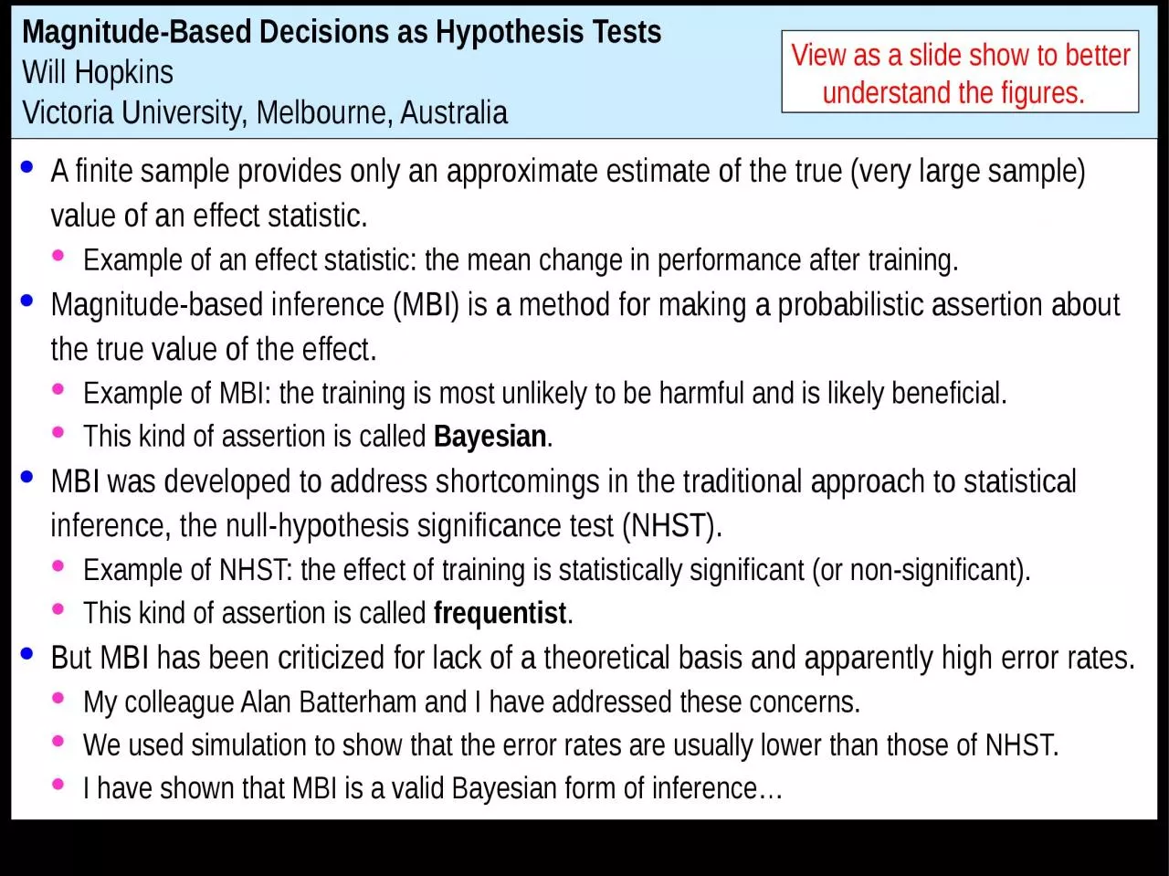
A finite sample provides only an approximate estimate of the true (very large sample) - PowerPoint Presentation

Slide1

A finite sample provides only an approximate estimate of the true (very large sample) value of an effect statistic.Example of an effect statistic: the mean change in performance after training.Magnitude-based inference (MBI) is a method for making a probabilistic assertion about the true value of the effect.Example of MBI: the training is most unlikely to be harmful and is likely beneficial.This kind of assertion is called Bayesian.MBI was developed to address shortcomings in the traditional approach to statistical inference, the null-hypothesis significance test (NHST).Example of NHST: the effect of training is statistically significant (or non-significant).This kind of assertion is called frequentist.But MBI has been criticized for lack of a theoretical basis and apparently high error rates. My colleague Alan Batterham and I have addressed these concerns.We used simulation to show that the error rates are usually lower than those of NHST.I have shown that MBI is a valid Bayesian form of inference…

Magnitude-Based Decisions as Hypothesis TestsWill HopkinsVictoria University, Melbourne, Australia

View as a slide show to better understand the figures.

Bayesian analyses require inclusion of a prior belief or information about the uncertainty in the magnitude of the effect.The assertions in MBI are equivalent to those of a Bayesian analysis in which the prior is practically uninformative.Some vociferous frequentist statisticians were still not convinced about MBI.The statistician Sander Greenland therefore advised showing that MBI is equivalent to hypothesis testing. In the hypothesis-testing view, having an hypothesis to reject is fundamental to the scientific method.And hypothesis testing has well-defined error rates.Greenland also thinks inference should be reserved for a conclusion about an effect that takes into account all sources of uncertainty, not just sampling variation (uncertainty arising from the finite size of a sample).Example: the sample may not be representative of a population.

Example: the model (equations or formulae) you use to derive the effect may be unrealistic.MBI and NHST deal only with sampling variation.MBI has therefore been rebranded as magnitude-based decisions (MBD).I show here that the decision process and errors in MBD are equivalent to those of several hypothesis tests.

Hypothesis TestsAn hypothesis test is conducted by calculating a probability (p) value representing evidence against the hypothesis. The smaller the p value, the more unlikely the hypothesis, so the better the evidence against the hypothesis. With a sufficiently small p value, you reject the hypothesis. Example: the classic p value used in NHST.NHST is a way of determining whether the value of an effect in a sample is so unlikely, given the hypothesis of no effect (the null hypothesis, H0), you can conclude the effect is not null; that is, you can reject the null hypothesis. The differences between the individual values in the sample can be used to derive the distribution representing the expected variation in the mean

with repeated sampling, if H0 is true.If the sample mean falls in the region of extreme valuesthat have a low probability (p=0.05), there is sufficient evidence against the null

.

That is, H

0 is rejected, and the effect is said to bestatistically significant.

e

xtreme values with

low

probability (p=0.05

)

p =

0.025

p =

0.025

value

of the

effect

0

probability

H

0

But statisticians can perform the null-hypothesis test in a different manner.They draw a probability distribution centered on the observed sample value:The distribution represents effect values that are compatible with the data and model.The 95% compatibility interval (formerly, 95% confidence interval) represents the 95% of values that are most compatible with the data and the model.The interval here includes zero, so the data and model are compatible with a true effect of zero, so the null hypothesis H0 cannot be rejected.Here are the same data illustrating how the classic p value is calculated.The p value for the test is 0.04 + 0.04 = 0.08, as shown.P is >0.05, so the data and model do not support rejection of H0.In the third figure,

the data and model are not compatible with H0: the 95%CI does not include 0; equivalently the p value is <0.05 (0.01 + 0.01 = 0.02), so H0 is rejected.

0

p =

0.01

p =

0.01

0

p =

0.04

p =

0.04

H

0

p =

0.025

observed value

0

p =

0.025

H

0

probability

95%CI

area

= 95%

The Bayesian interpretation of the 95%CI is the range in which the true effect is 95% likely to fall.If the range includes zero, the true effect "could be" zero. Of course, no effect can be exactly any value, so it is incorrect to say that the true effect could be zero. However, it is equally incorrect to state an hypothesis that the true effect is zero, because no effect can ever have a true value of exactly zero. So a point value for an hypothesis is unrealistic.For an effect that is relevant in a clinical or practical setting, it is important to avoid implementing a harmful effect.Harmful means the opposite of beneficial, not side effects. The hypothesis that the true effect could be harmful is therefore a more relevant hypothesis to reject than the null. A test of this kind

belongs to the class of one-sided interval-hypothesis testsRejection of this hypothesis allows the researcher to move toward an understanding and a decision about the effect.

The Hypothesis that the True Effect is HarmfulHere are examples of distributions, compatibility intervals and p values that could occur with samples.The purple region defines H0: all values to the left of the smallest harmful value.Harmful values are compatible with the sample and model, if the compatibility interval includes harmful values.The hypothesis of harm is therefore not rejected in the first example. The p value for the test is 0.06.The threshold p value is 0.025, if a 95% compatibility interval is used for the test.The second example allows rejection with a 95% interval: p=0.02, which is <0.025.The third example allows rejection with a 99% interval: p=0.004, which is <0.005.

0

p =

0.02

95%CI

0

p =

0.004

99%CI

95%CI

0

probability

smallest harmful value

0

H

95%CI

0.06

p =

observed

value

The threshold p value defines the maximum error rate for rejecting the hypothesis of harm, when the true effect is marginally harmful. The rate is set by the researcher through the choice of level of compatibility interval, similar to setting the error rate for rejecting the null hypothesis when the true effect is 0.For a 99% compatibility interval, the p-value threshold is 0.005.The probability of making an error is 0.005, and the error rate is 0.005*100 = 0.5%.This figure shows why:This error rate is independent of sample size.

The error here is a Type-2, or false negative, or failed discovery, since the researcher is erroneously rejecting an hypothesis that the true effect is substantial (harmful).

H

0

Sampling

distribution for

an

observed effect giving marginal

rejection

of

H

0

smallest

probability

0

harmful value

observed value for

marginal rejection of H

0

area =

0.005

Sampling

distribution

when

the true effect

is

the

smallest harmful

observed values

for rejection of H

0

p

H

=

0.005

Error rate

= 0.005*100

= 0.5%

In the clinical version of MBD, the p value for the test of harm is given a Bayesian interpretation: the probability that the true effect is harmful.An effect is considered for implementation when the probability of harm is <0.005 (<0.5%). This requirement is therefore equivalent to rejecting the hypothesis of harm with p<0.005 in a one-sided interval test.This equivalence holds, even if the Bayesian interpretation is not accepted by frequentists and strict Bayesians, because the probability of harm in MBD is calculated in exactly the same way as the p value for the test.MBD is still apparently the only approach to inferences or decisions in which an hypothesis test for harm, or equivalently the probability of harm, is the primary consideration in design and analysis.Does p<0.005 represent reasonable evidence against the hypothesis of harm…?

Does p<0.005 represent reasonable evidence against the hypothesis of harm?Greenland supports converting p values to S or "surprisal" values.The S value is the number of consecutive heads in coin tossing that would have the same probability as the p value. The S value is given by ‑log2(p), and with p=0.005, the value is 7.6 head tosses. So, saying that the treatment is not compatible with harmful values, when the p value is <0.005, carries with it a risk that the treatment is actually harmful, and the risk is equivalent to tossing >7.6 heads in a row, which seems quite rare. I am unaware of a scale for S values, but I deem p<0.005 to be most unlikely. The only other researchers using a qualitative scale for probabilities comparable to that of MBD is the panel of experts convened for the Intergovernmental Panel on Climate Change (IPCC), who deem p<0.01 (i.e., S>6.6) to be exceptionally unlikely. With a threshold for harm of half this value, MBD is one coin toss more conservative.P<0.005 can also be expressed as less than one event in 200 trials, which may be a better way to consider the error rate or the risk of harm than

coin tossing.

The Hypothesis that the True Effect is BeneficialMaking a decision about implementation of a treatment is more than just using a powerful test for rejecting the hypothesis of harm.Bayesian interpretation: ensuring a low risk of implementing a harmful effect. There also needs to be consideration that the treatment could be beneficial. Another one-sided test is involved.  Here are two examples. I have deliberately omitted the level of the compatibility interval.

0

smallest beneficial value

H

0

p

0

probability

In the first example, the compatibility interval falls short of the smallest beneficial value.No beneficial values are consistent with the data and model.So you reject the hypothesis that the effect is beneficial, and you would not implement it.Bayesian interpretation: the p value is the chance that the true effect is beneficial, and it is too low to implement it.

In the second example, the compatibility interval overlaps beneficial values.Beneficial values are compatible with the sample and model.So you cannot reject the hypothesis that the effect is beneficial; you could implement it.

Bayesian interpretation: there is a reasonable chance

that the true effect is

beneficial, so you could implement it.

0

smallest beneficial value

H

0

p

0

probability

But what level should the researcher choose for the compatibility interval and the associated threshold p value? In the calculation of sample size for NHST with 80% power, it is a 60% confidence interval.The probability distribution of the effect when the observed value is marginally significant has a right-hand tail overlapping the smallest beneficial effect with a probability of 0.20.Equivalently, there is 80% power or a probability of 0.80 of getting significance when the true effect is the smallest beneficial. Partly for this reason, the level of the compatibility interval for MBD is similar, 50%. This value was chosen originally via the Bayesian interpretation: the p value represents the chance that the true effect is beneficial.With a 50

% interval, the tail is 25%, which is interpreted as possibly beneficial. That is, you would consider implementing an effect that is possibly beneficial, provided there is a sufficiently low risk of harm.

Feel free to specify

a higher level

for the compatibility interval for benefit, to reduce the error rate for rejecting the beneficial hypothesis, when the true effect is beneficial. But beware! For example, if a 90% interval is chosen, a tail overlapping into the beneficial region with an area of only 6% is regarded as failure to reject the beneficial hypotheses.

Or from the Bayesian perspective, an observed quite trivial effect with a chance of benefit of only 6% would be considered potentially implementable! And if the true effect is actually marginally trivial, there is automatically a high error rate

of just under 95% for implementing a treatment that is not beneficial.

There is also a problem with requiring a high chance of benefit for implementation.Consider this example, a test resulting in rejection of the hypothesis that the effect is not beneficial. If the p value for this test is the same as for the test for benefit, 0.05 say (for a one-sided 90% interval), then a marginally beneficial effect would be implemented only 5% of the time, regardless

of the sample size!So the MBD default of 0.25 (25%) is about right.There is a less conservative version of clinical MBD,

in which an

effect with a risk of harm >0.5% (or p value for the test of harm >0.005)

is considered potentially implementable, if the chance of benefit is high enough.The idea is that the

chance of benefit outweighs the risk of harm."High enough" is determined with an odds ratio: (odds of benefit)/(odds of harm), where odds = p/(1-p) or 100*p/(100-100*p).The threshold odds ratio corresponds to the marginally implementable finding of 25% chance of benefit and 0.5% risk of harm: 25/(100-25)/(0.5/99.5) = 66.3.

So an unclear effect with odds ratio >66.3 can be considered for implementation.It has higher error rates. The strict frequentist statisticians hate it.

0

Non-clinical MBD as Hypothesis TestsClinical MBD is used when an effect could result in a recommendation to implement a treatment.Example: a new training strategy, which might impair rather than enhance performance compared with current best practice.Implementing a harmful effect is more serious than failing to implement a beneficial effect. Hence, with clinical MBD, the two one-sided tests differ in their threshold p values.Non-clinical MBD is used when an effect could not result in implementation of a treatment.Example: mean performance of girls vs boys. If you find a substantial difference, you are not going to recommend a sex change.Non-clinical (or mechanistic) MBD is equivalent to two one-sided tests with the same threshold p values.A p value of 0.05, corresponding to one tail of a 90% compatibility interval, was chosen originally for its Bayesian interpretation: rejection

of the hypothesis of one of the substantial magnitudes corresponds to a chance of <5% that the true effect has that substantial magnitude, which is interpreted as very unlikely.

Combining the Two Hypothesis TestsFailure to reject both hypotheses results in an unclear (indecisive, inconclusive) outcome.The CI spans both smallest important thresholds, so the effect "could" be beneficial and harmful, or substantially +ive and –ive:(For a clinical effect, the CI is 99% on the harm side and 50% on the benefit side.)Unclear outcomes occur more often with smaller sample sizes, because the compatibility intervals are wider.Unclear outcomes do not contribute to error rates; they have their own indecisive rate.A study will be difficult to publish if the main outcome is unclear.Sample size is estimated for the worst-case scenario of marginal rejection of both

hypotheses, to avoid any unclear outcomes, whatever the true effect.The resulting minimum desirable sample size is practically identical for clinical and non-clinical effects.

Value of effect statistic

substantial positive

substantial negative

trivial

Only one hypothesis needs to be rejected for publishability.Example: this effect "could be" positive or trivial (cannot reject hypothesis of positive), but it can't be negative (reject hypothesis of negative):The effect has adequate precision or acceptable uncertainty (formerly a clear effect).Simulations show that publishing such findings does not result in substantial upward publication bias in magnitudes, even with quite small sample sizes.Publication of statistically significant effects with small sample sizes does result in bias.An effect is decisively substantial if the 90%CI falls entirely in substantial values.

Example: this effect cannot be negative or trivial (reject hypotheses of negative and trivial); it can only be positive:This effect is clearly

(decisively, conclusively) positive, or very likely positive, or moderately compatible with substantial positive values.

Value of effect statistic

substantial positive

substantial negative

trivial

Value of effect statistic

substantial positive

substantial negative

trivial

Rejection of both hypotheses (benefit and harm, or substantial +ive and –ive) implies that the effect could only be trivial, inconsequential, unimportant or insignificant:But with a 90%CI that just fits in the trivial region, the effect is only likely trivial.For consistency with clearly positive meaning very likely positive, clearly trivial needs to be equivalent to very likely trivial.This corresponds to rejection of the non-trivial hypothesis using a 95%CI, not a 90%CI.A technical point not worth worrying about!

Value of effect statistic

substantial positive

substantial negative

trivial

Type-1 Errors in MBDA Type-1 error is a false positive or false discovery: a true trivial effect is deemed to be decisively non-trivial. In NHST, a significant effect is usually assumed to be substantial, so the Type-1 error rate for a truly zero effect is set to 5% by the p value for statistical significance.But the error rate approaches 80% for a marginally trivial true effect, depending on sample size.In clinical MBD, failure to reject the hypothesis of benefit is regarded as sufficient evidence to implement the effect.Therefore a Type-1 error occurs, if the true magnitude of the effect is trivial.With a threshold p value of 0.25, Type-1 error rates approach 25% for a true zero effect and 75% for marginally trivial true effects, depending on sample size.

Most of these errors occur with effects that are presented as possibly or likely beneficial, so the practitioner should be in no doubt about the modest level of evidence for the effect being beneficial.In non-clinical MBD, erroneous rejection of the trivial hypothesis is a Type-1 error.

That is, the 90%CI has to fall entirely in substantial values.

The resulting Type-1 error rate seldom exceeds 5% and never exceeds 10%.

More-Conservative P-value Thresholds?The non-clinical threshold of 0.05 seems reasonable, expressed as one event in 20 trials. But expressed as an S value, it represents only a little more than four heads in a row. An advantage of 0.05 is approximately the same sample size as for clinical MBD. If this threshold were revised downward, non-clinical sample size would be greater than that for clinical, which seems unreasonable.So the probability thresholds in clinical MBD would also need revising downwards.For example, halve all the p-value thresholds?For non-clinical MBD, very unlikely (0.05 or 5%) would become 0.025 or 2.5%, and the S value would move up by one coin toss to 5.3.For clinical MBD, most unlikely (0.005 or 0.5%) would become 0.0025 or 0.25%, and possibly (0.25 or 25

%) would become 0.125 or 12.5%. The S values would increase to 8.6 and 3.0 heads in a row. Sample size for clinical and non-clinical MBD would still be practically the same and almost exactly one-half (instead of one-third) those of NHST for 5% significance and 80% power. But smaller p values require bigger effects for a given sample size, so there could be a risk of substantial bias with smaller threshold p

values when the sample size is small.

Sport

scientists would also have fewer publishable outcomes with some of their unavoidably small sample sizes.

You have been warned!

Reporting MBD Outcomes Some journals will be happy with Bayesian terms to describe of the uncertainty in the magnitude of an effect as uncertainty in the true value.Example: the effect of the treatment is likely beneficial (and most unlikely harmful).Others will prefer frequentist descriptions of the uncertainty that reflect the underlying hypothesis tests.Example: the effect of the treatment is weakly compatible with benefit (and harm is strongly rejected).This table summarizes the correspondence of the terms:

Some journals may require presentation of pB and pH, p+ and p

–

, and

pT.All journals should require presentation of compatibility limits, preferably 90%.

Chances

<0.5%

Bayesian termmost unlikely0.5-5%very unlikely

P value

<0.005strongly rejectFrequentist term0.005-0.05moderately reject0.05-0.25

5-25%

unlikely

weakly reject

0.25-0.7525-75%possiblyambiguously compatible0.75-0.9575-95%likelyweakly compatible>0.995>99.5%most likely0.95-0.995

95-99.5%very likelymoderately compatiblestrongly compatible

The following two slides introduce two relevant Sportscience spreadsheets.Converting P Values to Magnitude-Based DecisionsStatistical significance is on the way out, but the associated classic p values will be around for years to come.The p value alone does not provide enough information about the uncertainty in the true magnitude of the effect.To get the uncertainty expressed as compatibility limits or interval, you need also the sample value of the effect.Put the p value and sample value into the spreadsheet Convert p values to MBD.The upper and lower limits of the compatibility interval tell you how big or small the true effect could be, numerically.But are those limits important? To answer that, you need to know the smallest important value of the effect. You can then see whether the compatibility limits are important to decide how important the effect could be.

That’s OK for non-clinical effects, but if the effect represents a treatment or strategy that could be beneficial or harmful, you have to be really careful about avoiding harm.For such clinical effects, it’s better to work out the chances of harm and benefit before you make a decision about using the effect.

Even for non-clinical effects, it’s important to know the chances that the effect is substantial (and trivial).

And if there is too much uncertainty, you have to decide that the effect is unclear.More data are needed to reduce the uncertainty.The spreadsheet works out the likelihoods from the p value, the sample value of the effect, and the smallest important effect. Deciding on the smallest important is not easy. See Lectures 4, 5 and 10.The spreadsheet has frequentist and Bayesian versions.Converting Compatibility Intervals into Magnitude-Based DecisionsSome authors no longer provide p values, or they may provide only an unusable p-value inequality: p>0.05.If they provide p<0.05, you can do MBD by assuming p=0.05.But if they provide compatibility intervals or limits, you can do MBD.Once again you need the smallest important value of the effect.

You could use the previous spreadsheet, by trying different p values to home in on the same compatibility limits.Or a spreadsheet designed to Combine/compare

effects

can be used to derive the magnitude-based

decision for a single effect.A spreadsheet in this workbook also does a Bayesian analysis with an informative prior.

You have to provide prior information/belief about the effect as a mean and compatibility limits.The spreadsheet shows that realistic weakly informative priors produce a posterior compatibility interval that is practically the same as the original, for effects with the kind of CI you get with the usual small samples in sport research. Read the article on the Bayesian analysis

link for more.