Frequent Itemsets The Market-Basket Model - PowerPoint Presentation

Slide1

Frequent Itemsets

The Market-Basket ModelAssociation RulesA-Priori AlgorithmOther Algorithms

Jeffrey D. Ullman

Stanford UniversitySlide2

2The Market-Basket ModelA large set of items, e.g., things sold in a supermarket.A large set of baskets

, each of which is a small set of the items, e.g., the things one customer buys on one day.Slide3

3SupportSimplest question: find sets of items that appear “frequently” in the baskets.Support for

itemset I = the number of baskets containing all items in I.Sometimes given as a percentage of the baskets. Given a support threshold s, a set of

items appearing in at least s baskets is called a

frequent

itemset

.Slide4

4Example: Frequent ItemsetsItems={milk, coke,

pepsi, beer, juice}.Support = 3 baskets. B1 = {m, c, b} B2 = {m, p, j} B3 = {m, b} B4 = {c, j} B

5 = {m, p, b} B6 = {m, c, b, j} B

7

= {c, b, j} B

8

= {b, c}

Frequent

itemsets

: {m}, {c}, {b}, {j},

, {

b,c

}

, {

c,j

}.

{m,b}Slide5

Applications“Classic” application was analyzing what people bought together in a brick-and-mortar store.Apocryphal story of “diapers and beer” discovery.Used to position potato chips between diapers and beer to enhance sales of potato chips.Many other applications, including plagiarism detection.Items = documents; baskets = sentences.Basket/sentence contains all the items/documents that have that sentence.

5Slide6

6Association RulesIf-then rules about the contents of baskets.{i

1, i2,…, ik} → j

means: “if a basket contains all of i1,…, i

k

then it is

likely

to

contain

j

.”

Example

: {bread, peanut-butter} → jelly.Confidence of this association rule is the “probability” of j given i1

,…, ik.That is, the fraction of the baskets with i1,…, ik that also contain j

.Subtle point: “probability” implies there is a

process generating random baskets. Reallywe’re just computing the fraction of baskets,because we’re computer scientists, not statisticians.Slide7

7Example: Confidence B1

= {m, c, b} B2 = {m, p, j} B3 = {m, b} B4 = {c, j} B5 = {m, p, b} B6 = {m, c, b, j} B7 = {c, b, j} B

8 = {b, c}An association rule: {m, b}

→

c

.

Confidence = 2/4 = 50%.

+

_

_ +Slide8

8Computation ModelTypically, data is a file consisting of a list of baskets.The

true cost of mining disk-resident data is usually the number of disk I/O’s.In practice, we read the data in passes – all baskets read in turn.Thus, we measure the cost by the number of passes an algorithm takes.Slide9

9Main-Memory BottleneckFor many frequent-itemset algorithms, main memory is the critical resource.As we read baskets, we need to count something, e.g., occurrences of pairs of items.

The number of different things we can count is limited by main memory.Swapping counts in/out is a disaster.Slide10

10Finding Frequent PairsThe hardest problem often turns out to be finding the frequent pairs.Why

? Often frequent pairs are common, frequent triples are rare.Why? Support threshold is usually set high enough that you don’t get too many frequent itemsets.We’ll concentrate on pairs, then extend to larger sets.Slide11

11Naïve AlgorithmRead file once, counting in main memory the occurrences of each pair.From each basket of n items, generate its

n(n-1)/2 pairs by two nested loops.Fails if (#items)2 exceeds main memory.Example: Walmart sells 100K items, so probably OK.Example: Web has 100B pages, so definitely not OK.Slide12

122 Approaches to Main-Memory CountingCount

all pairs, using a triangular matrix.I.e., count {i,j} in row i, column j, provided i < j.But use a “ragged array,” so the empty triangle is not there.Keep a table of triples [i, j

, c] = “the count of the pair of items {i, j}

is

c

.”

(1) requires only 4 bytes/pair.

Note

: always assume integers are 4 bytes.

(2) requires

at least 12

bytes/pair,

but only for those pairs with count > 0

.

I.e., (2) beats (1) only when at most 1/3 of all pairs have a nonzero count.Slide13

134 per pair

Triangular matrix

Tabular method

12

12 per point

per

occurring pairSlide14

14One-Dimensional Representation of a Triangular ArrayNumber items 1, 2,…,

n.Requires table of size O(n) to convert item names to consecutive integers.Count {i, j} only if i < j. Keep pairs in the order {1,2}, {1,3},…, {

1,n}, {2,3}, {2,4

},…, {2,

n

},

{3,4},…, {

3,

n

},…, {

n

-

1,

n

}.Find pair {i, j}, where i<j, at the position:

(i – 1)(n – i/2) + j

– iTotal number of pairs n(n –1)/2; total bytes about 2n2.Slide15

The A-Priori Algorithm

Monotonicity of “Frequent”Candidate PairsExtension to Larger ItemsetsSlide16

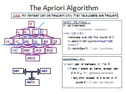
16A-Priori AlgorithmA two-pass approach called a-priori limits the need for main memory.

Key idea: monotonicity: if a set of items appears at least s times, so does every subset of the set.Contrapositive for pairs: if item i does not appear in s

baskets, then no pair including i can appear in s baskets

.Slide17

17A-Priori Algorithm – (2)Pass 1: Read baskets and count in main memory the occurrences of each item.Requires only memory proportional to #items.Items that appear at least

s times are the frequent items.Slide18

18A-Priori Algorithm – (3)Pass 2: Read baskets again and count in main memory only those pairs both of which were found in Pass 1 to be frequent.Requires memory proportional to square of

frequent items only (for counts), plus a table of the frequent items (so you know what must be counted).Slide19

19Picture of A-Priori

Item counts

Pass 1

Pass 2

Frequent items

Counts of

pairs of

frequent

itemsSlide20

20Detail for A-PrioriYou can use the triangular matrix method with n = number of frequent items.May save space compared with storing triples.

Trick: number frequent items 1, 2,… and keep a table relating new numbers to original item numbers.Slide21

21A-Priori Using Triangular Matrix

Item counts

Pass 1

Pass 2

Old #’s New #’s

1

-

2

Counts of

pairs of

frequent

items

For thought

: Why would we even

mention the infrequent items?Slide22

22Frequent Triples, Etc.For each size of itemsets k, we construct two sets of

k-sets (sets of size k):Ck = candidate k-sets = those that might be frequent sets (support

> s) based on information from the pass for itemsets

of size

k

– 1

.

L

k

= the set of truly frequent

k

-sets

.Slide23

23

C1

L1

C

2

L

2

C

3

Filter

Filter

Construct

Construct

First

pass

Second

pass

All

items

All pairs

of items

from L

1

Count

the pairs

To be

explained

Count

the items

Frequent

items

Frequent

pairsSlide24

24Passes Beyond TwoC1 = all itemsIn general, L

k = members of Ck with support ≥ s.Requires one pass.Ck+1 = (k+1)-sets, each

k of which is in Lk

.

For thought

: how would you generate

C

k

+1

from

L

k

?

Enumerating all sets of size k+1 and testing each seems really dumb.Slide25

Memory RequirementsAt the kth pass, you need space to count each member of Ck.In realistic cases, because you need fairly high support, the number of candidates of each size drops, once you get beyond pairs.

25Slide26

The PCY (Park-Chen-Yu) Algorithm

Improvement to A-PrioriExploits Empty Memory on First PassFrequent BucketsSlide27

27PCY AlgorithmDuring Pass 1 of A-priori, most memory is idle.Use that memory to keep counts of buckets into which pairs of items are hashed.

Just the count, not the pairs themselves.For each basket, enumerate all its pairs, hash them, and increment the resulting bucket count by 1.Slide28

28PCY Algorithm – (2)A bucket is frequent if its count is at least the support threshold.If a bucket is not frequent, no pair that hashes to that bucket could possibly be a frequent pair.

On Pass 2, we only count pairs of frequent items that also hash to a frequent bucket.A bitmap tells which buckets are frequent, using only one bit per bucket (i.e., 1/32 of the space used on Pass 1).Slide29

29Picture of PCY

Hash tablefor pairs

Item counts

Bitmap

Pass 1

Pass 2

Frequent items

Counts of

candidate

pairsSlide30

30Pass 1: Memory OrganizationSpace to count each item.One (typically) 4-byte integer per item.Use the rest of the space for as many integers, representing buckets, as we can.Slide31

31PCY Algorithm – Pass 1FOR (each basket) {

FOR (each item in the basket) add 1 to item’s count; FOR (each pair of items) { hash the pair to a bucket; add 1 to the count for that bucket

}

}Slide32

32Observations About BucketsA bucket that a frequent pair hashes to is surely frequent.We cannot

eliminate any member of this bucket.Even without any frequent pair, a bucket can be frequent.Again, nothing in the bucket can be eliminated.But if the count for a bucket is less than the support s, all pairs that hash to this bucket can be eliminated,

even if the pair consists of two frequent items.Slide33

33PCY Algorithm – Between PassesReplace the buckets by a bit-vector (the “bitmap”):

1 means the bucket is frequent; 0 means it is not.Also, decide which items are frequent and list them for the second pass.Slide34

34PCY Algorithm – Pass 2Count all pairs {i, j} that meet the conditions for being a

candidate pair:Both i and j are frequent items.The pair {i, j}, hashes to a bucket number whose bit in the bit vector is

1.Slide35

35Memory DetailsBuckets require a few bytes each.Note: we don’t have to count past s.

If s < 216, 2 bytes/bucket will do.# buckets is O(main-memory size).On second pass, a table of (item, item, count) triples is essential.Thus, hash table on Pass 1 must eliminate 2/3 of the candidate pairs for PCY to beat a-priori.Slide36

More Extensions to A-PrioriThe MMDS book covers several other extensions beyond the PCY idea: “Multistage” and “Multihash.”For reading on your own, Sect. 6.4 of MMDS.Recommended video (starting about 10:10):

https://www.youtube.com/watch?v=AGAkNiQnbjY36Slide37

All (Or Most) Frequent Itemsets In

< 2 PassesSimple AlgorithmSavasere-Omiecinski- Navathe

(SON) AlgorithmToivonen’s AlgorithmSlide38

38Simple AlgorithmTake a random sample of the market baskets.

Do not sneer; “random sample” is often a cure for the problem of having too large a dataset.Run a-priori or one of its improvements (for sets of all sizes, not just pairs) in main memory, so you don’t pay for disk I/O each time you increase the size of itemsets.Use as your support threshold a suitable, scaled-back number.Example: if your sample is 1/100 of the baskets, use s/100 as your support threshold instead of

s.Slide39

39Simple Algorithm – OptionOptionally, verify that your guesses are truly frequent in the entire data set by a second pass.But you don’t catch sets frequent in the whole but not in the sample.

Smaller threshold, e.g., s/125 instead of s/100, helps catch more truly frequent itemsets.But requires more space.Slide40

40SON AlgorithmPartition the baskets into small subsets.Read each subset into main memory and perform the first pass of the simple algorithm on each subset

.Parallel processing of the subsets a good option.An itemset is a candidate if it is frequent (with support threshold suitably scaled down) in at least one subset.Slide41

41SON Algorithm – Pass 2On a second pass, count all the candidate itemsets and determine which are frequent in the entire set.

Key “monotonicity” idea: an itemset cannot be frequent in the entire set of baskets unless it is frequent in at least one subset.Slide42

42Toivonen’s AlgorithmStart as in the simple algorithm, but lower the threshold slightly for the sample.Example: if the sample is 1% of the baskets,

use s/125 as the support threshold rather than s/100.Goal is to avoid missing any itemset that is frequent in the full set of baskets.Slide43

43Toivonen’s Algorithm – (2)Add to the itemsets that are frequent in the sample the negative

border of these itemsets.An itemset is in the negative border if it is not deemed frequent in the sample, but all its immediate subsets are.Immediate subset

= “delete exactly one element.”Slide44

44Example: Negative Border{A

,B,C,D} is in the negative border if and only if:It is not frequent in the sample, butAll of {A,B,

C}, {B,C,

D

},

{

A

,

C

,

D

}, and

{

A

,B,D} are. {A} is in the negative border if and only if it is not frequent in the sample.Because the empty set is always frequent.Unless there are fewer baskets than the support threshold (silly case).

Useful trick: When processing the sample by A-Priori, each member of Ck is either in Lk or in the negative border, never both.Slide45

45Picture of Negative Border

…tripletonsdoubletonssingletons

Negative Border

Frequent Itemsets

from SampleSlide46

46Toivonen’s Algorithm – (3)In a second pass, count all candidate frequent itemsets from the first pass, and also count sets in their negative border.

If no itemset from the negative border turns out to be frequent, then the candidates found to be frequent in the whole data are exactly the frequent itemsets.Slide47

47Toivonen’s Algorithm – (4)What if we find that something in the negative border is actually frequent?We must start over

again with another sample!Try to choose the support threshold so the probability of failure is low, while the number of itemsets checked on the second pass fits in main-memory.Slide48

48If Something in the Negative Border Is Frequent . . .

…tripletonsdoubletonssingletons

Negative Border

Frequent Itemsets

from Sample

We broke through the

negative border. How

far does the problem

go?Slide49

49Theorem:If there is an itemset that is frequent in the whole, but not frequent in the sample, then there is a member of the negative border for the sample that is frequent in the whole.Slide50

50Suppose not; i.e.;There is an itemset S frequent in the whole but not frequent in the sample, and

Nothing in the negative border is frequent in the whole.Let T be a smallest subset of S that is not frequent in the sample.T is frequent in the whole (

S is frequent + monotonicity).T is

in the negative border (else not “smallest”).

Proof

: