/
Probability Distribution Probability Distribution

Probability Distribution - PDF document

alyssa
alyssa . @alyssa
Follow
352 views
Uploaded On 2021-03-17

Probability Distribution - PPT Presentation

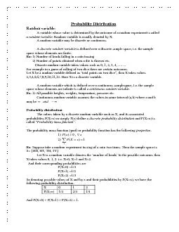
Random variable A variable whose value is determined by the outcome of a random experiment is called a random variable Random variable is usually denoted by X A random variable may be discrete or ID: 832059

probability random discrete variable random probability variable discrete function values variables defined independent distribution number find theorem joint expectation

Share:

Link:

Embed:

Download Presentation from below link

Download Pdf The PPT/PDF document "Probability Distribution" is the property of its rightful owner. Permission is granted to download and print the materials on this web site for personal, non-commercial use only, and to display it on your personal computer provided you do not modify the materials and that you retain all copyright notices contained in the materials. By downloading content from our website, you accept the terms of this agreement.


Presentation Transcript

Probability DistributionRandom variable
Probability DistributionRandom variable: A variable whose value is determined by the outcome of a random experiment is called a random variable. Random variable is usually denoted by X. A random variable may be discrete or continuous. A discrete random variable is defined over a discrete sample space, i.e. the sample space whose elements are finite. Ex: 1) Number of heads falling in a coin tossing 2) Number of points obtained when a die is thrown etc. Discrete random variable takes values such as 0, 1, 2, 3, 4, ……. For example in a game of rolling of two dice there are certain outcomes. Let X be a random variable defined as ‘total points on two dice”, then X takes values 2,3,4,5,6,7,8,9,10,11,12. Here X is a discrete variable. A random variable which is defined over a continuous samplespace, i.e. the sample space whose elements are infinite is called a continuous random variable. Ex: 1) All possible heights, weights, temperature, pressure etc. Continuous random variable assumes the values in some interval (a,b) where a and b may be ¥-¥andProbability distribution: The values taken by a discrete random variable such as X, and its associated probabilities P(X=x) or simply P(x) define a discrete probability dist

ribution and P(X=x) is called “Probabili
ribution and P(X=x) is called “Probability mass function”. . The probability mass function (pmf) or probability function has the following properties. 1) ³, " 2) ( Ex: Suppose take a random experiment tossing of a coin two times. Then the sample space is S= {HH, HT, TH, TT} Let X is a random variable denotes the ‘number of heads’ in the possible outcomes then X takes values 0, 1, 2. i.e. X=0, X=1 and X=2. And their corresponding probabilities are P(X=0) =1/4 P(X=1) =1/2 P(X=2) =1/4 So denoting possible values of X and by x and their probabilities by P(X=x), we have the following probability distribution. X 0 1 2 P(X=x) 1/4 2/4 1/4 And P(X=0) + P(X=1) + P(X=2) = 1. The values taken by a continuous random variable X, and its associated probabilities P(X=x) or simply P(x) define a continuous probability distribution and P(X=x) is called Probability density function” and it has following properties 1)0³, " ¥¥-x 2)dxMathematical Expectation: If X denotes a discrete random variable which can assume the values ,.....with respective probabilities ...,,........., where .The Mathematical Expectation of denoted by E(X) is defined as E(X) = Ex: 1) A coin is tossed two times. Find the mathematical exp

ectation of getting heads? Sol: Define X
ectation of getting heads? Sol: Define X as number of heads in tossing of two coins. So X takes values 0, 1, 2. And P(X=0) = 1/4 P(X=1) = 2/4 P(X=2) = 1/4 Now E(X) = = 4124214  E(X) =1. Ex: 2) A die is thrown once. Find the mathematical expectation of the point on the upper face of the die. Sol: Define a random variable X as the point on the upper face of the die. So X takes values 1, 2, 3, 4, 5, 6. The probability distribution is Now E(X) = 616615614613612611´+´+´+´+´+´ =5.3621X 1 2 3 4 5 6 P(X=x) 1/6 1/6 1/6 1/6 1/6 1/6 Def: The mathematical expectation of g(x) is defined as E [g(x)] = provided is finite Putting ()2,We get E [] = E [] = E [+] = )32(Theorem:1) If a and b are constants then E [ax+] = aE(x) + b Proof: E [ax+] = ax =axbp =aE (x) + b Theorem:2) If g(x) and h(x) are any two functions of a discrete random variable X, then E[g(x)± h(x)]= E[g(x)] ± E[h(x)] Proof: E [g(x)± h(x)]= )]] =± = E [g(x)] ± E[h(x)] Def: The ‘Variance’ of a random variable ‘X’ is given by )]]XEXE- Theorem:3) )]]XEXE-= E [X] - [E(X)]Proof: )]]XEXE-==±kiiixpXEx12)()]] =)]]-=kiiixpXEx1)()(2 = E [X] + )]]XE=kiixp1

)( -2 E [X = E [X] + )]]XE -2 E [
)( -2 E [X = E [X] + )]]XE -2 E [X] E [X] [=1] = E [X] - [E(X)]Theorem:4) If X is a random variable and a and b are constants then V [aX+] = V(X) . Proof: V [aX+] =)][(aXaX =)][(aEaX =)][(aEaX =))]]XEXaE- =)][( =V(X). Joint probability distribution: If X and Y are two discrete random variables, the probability for the simultaneous occurrence of X and Y can be represented by ()or (), then a joint probability distribution is defined by all the possible values of X and Y associated with the joint probability density function (). (X, Y) is said to be a two dimensional random variable. In discrete case () have the following properties i) 0³yxP "and ii) xy( Ex: If a coin is tossed two times Define X as the result on the first coin i.e. H , T Y as the result on the first coin i.e. H , T Now the joint probability distribution of X and Y can be constructed as below H T H 1/4 1/4 T 1/4 1/4 Marginal density function: Given that the joint probability function() of the discrete random variables X and Y, the marginal density function of x is defined as ( "x the marginal density function of y is defined as =xyxPyQ),()(

"yConditional probability function: Gi
"yConditional probability function: Given that the joint probability function() of the discrete random variables X and Y, the Conditional probability function of x given y is defined as =)/(yxP , )�0 the Conditional probability function of y given is defined as =)/(xyP , )�0 Where )and )are the marginal density functions of y and x respectively. X Y Independent random variables: Two discrete random variables X and Y are said to be independent if ()=)"andNote: In case of independent random variables =)/(yxP)(xP"and and =)/(xyP)(yP"andTheorem: If X and Y are two discrete random variables with joint probability function ()then E [g(X)± h(Y)] = E [g(X)] ± E [h(Y)]. Proof: E [g(x)± h(y)] =ij)](), = ij()jiyxP,±ij(), =iixg)(()ixP±jjyh)(()jyP[( (] = E [g(X)]± E [h(Y)] Similarly putting g(X)=X and h(Y)=Y in the above theorem we get E [X± Y] = E [X] ± E [Y]. Theorem: If X and Y are two independent discrete random

variables with joint probability functi
variables with joint probability function () then )XY=Proof: )XYij(), =ij() [X and Y are independent] =iix()ixPjjy() =)Covariance of X and Y: Covariance of X and Y is written symbolically as Cov(X, Y) or XY and is defined as Cov(X, Y) = )])][-- And Cov(X, Y) = )])][-- =)]]YEXEYXEYEXY+-- ==YEXEYEXEXEYEXY+-- =))YEXEXY- Theorem: If X and Y are independent then Cov(X, Y) = 0 Proof: If X and Y are independent then we have )XY= =�0=-XY =� Cov(X, Y) = 0 Theorem: If X and Y are two discrete random variables, then abCovbYaXProof: =+bYaX)][(bYaXbYaX)][(bEaEbYaX)}])}}YEYbXEXaE-+- =)}])}{)})}}2222YEYXEXab)])][[2)]])]]2222YEYXEXabE=)abCovNote: If X and Y are independent then )bYaX Cov(X, Y) = 0] Correlation coefficient: If )and )exist, the correlation coefficient (is measure of relationship) between X and Y is defined as Cov =)]])]])])][--The sign of ris determined by the sign of Cov

(X, Y) Note: If two variables X and Y ar
(X, Y) Note: If two variables X and Y are independent thenr=0 and X and Y are said to be uncorrelated. EXCERSICE1)Let X be a random variable having the following probability distribution. Find the expected values and the variance of i) X ii) 2X+1 iii) 2X-3 2)X is a randomly drawn number from the set {1,2,3,4,5,6,7,8,9,10}. Find E(2X-3). 3)X and Y are independent random variables with V(X) = V(Y) = 4. Find V(3X-2Y). 4)A bowl contains 6 chits, with numbers 1,2 and 3 written on two, three and one chits respectively. If X is the observed number on a randomly drawn chit, find E(X). 5)Define independence of two random variables. For independent random variables X and Y, assuming the addition and multiplication law of expectation, prove that bYaX6)Let us consider the experiment of tossing an honest coin twice. The random variable X takes values 0 or 1 according as head or tail appears at the result of the first toss. The random variable Y takes values either 0 or 1 according as whether head or tail appears as a result of second toss. Show that X and Y are independent. 7)Ram and Shyam alternately toss a die, Ram starting the process. He who throws 5 or 6 first gets a prize of Rs.10 and the game ends with the a

ward of the prize. Find the expectation
ward of the prize. Find the expectation of the Ram’s gain. 8)Clearly explain the conditions under which, )XY=also prove the relation. 9)In a particular game a gambler can win a sum of Rs.100 with probability 2/5 and lose a sum of Rs.50 with probability 3/5. What is the mathematical expectation of his gain. 10)A business concern consists of 5 senior level and 3 junior level executives. A committee is to be formed by taking 3 executives at random. Find the expected number of senior executives to be in the committee. 11)There are two boxes: a white colored box and a red colored box. Each box contains 3 balls marked 1, 2, and 3. One ball is drawn from each box and their numbers are marked. Let X denotes the number observed from white box and Y denotes the number observed from the red box. Show that i) E(X+Y) = E(X) +E(Y) ii) E (XY) = E(X) E(Y) iii) V(X+Y) = V(X) + V(Y) 12)Calculate the mean and the standard deviation of the distribution of random digits, that is, f(X) = 1/10, X=0,1,2,…….,9 13)A person picks up 4 cards at random from a full deck. If he receives twice as many rupees as the number of aces he gets, find the expected gain. X 1 2 3 4 5 P(X=x) 1/6 1/3 0