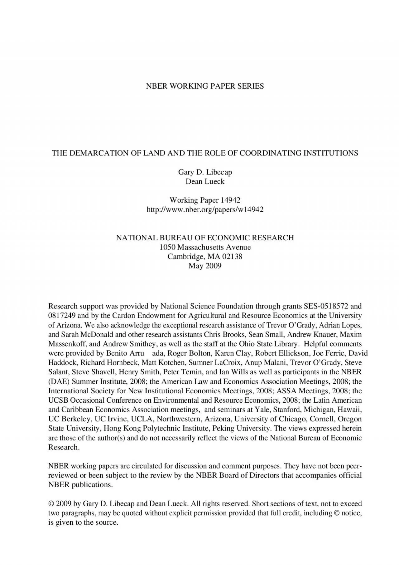
The Demarcation of Land and the Role of Coordinating InstitutionsGary - PDF document

The Demarcation of Land and the Role of Coordinating InstitutionsGary D. Libecap and Dean LueckABSTRACTThis paper examines the origins and economic effects of the two dominant land demarcation systems:Gary D. LibecapBren School of Environmental ScienceDean LueckDepartment of Agricultural and Resource EconomicsProgram on Economics, Law and the EnvironmentUniversity of Arizona 1 “The beauty of the land survey…was that it made buying simple, whether by squatter, settler or speculator. The system gave every parcel of virgin ground a unique identity, beginning with the township. Within the township, the thirty-six sections were numbered …, beginning with section 1 in the north-east corner, and continuing first westward then eastward, back and forth,….And long before the United States Postal Service ever dreamed of zip codes, every one of these quarter-quarter sections had its own address, as in ¼ South-West, ¼ Section North-West, Section 8, Township 22 North, Range 4 West, Fifth Principal Meridian.” (Rectangular Survey in Linklater, 2002, 180-81)“Beginning at a white oak in the fork of four mile run called the long branch & running No 88o Wt three hundred thirty eight poles to the Line of Capt. Pearson, then with the line of Person No 34 Et One hundred Eighty-eight poles to a Gum on the So Wt side of the run corner to persons red oak & chestnut land.” (Metes and Bounds in C.W. Stetson, 1935, 90). I. NTRODUCTIONThe demarcation of land is one of the earliest human activities. Demarcation began with territories to hunting and gathering sites, as well as early urban settlements, and in modern societies land is demarcated for residential and commercial use, for farmland, for offshore mineral exploitation, for wilderness landscapes, and many other purposes. It is a fundamental institution for defining property b

oundaries and location and in facilitating the market for land. While it seems self-evident that a system of demarcating rights to land will have long-term effects on land use and value, the literatures in economics and in law have not addressed these issues.1 In this paper we examine the origins and effects of the two dominant land demarcation systems: metes and bounds (MB) and the rectangular system (RS). MB has low initial setup costs, but fails to provide coordination among agents, implying that there will be relatively higher adjustment and transaction costs in the future. Under MB land is demarcated by local, natural features (trees, streams, rocks) and relatively permanent human structures (walls, bridges, monuments). Parcels are described independently by perimeter and linked to a specific survey within 1 We find no legal or economic scholarship on this topic and even major property law treatises (e.g., Dukeminier and Krier 2002, Merrill and Smith 2007) merely describe the dominant American system. Neither of the comprehensive treatises on law and economics by Posner (2002) and Shavell (2007) mentions land demarcation. Holmes and Lee (2008, 2009) make reference to spatial issues regarding land use, but do not examine the underlying demarcation structure. 2 a local political jurisdiction. Individuals take little account of the spatial and temporal impacts of their choices. Demarcation is vague and imprecise (“four paces from the most northerly rock pile…”) and idiosyncratic. There are no uniform addresses, boundaries, shapes, sizes, or alignments. A centralized and coordinated RS is a network that has higher upfront costs of implementation compared to MB because of systematic survey prior to occupancy. RS, however, defines land ownership in a manner that reduces the subsequent costs of measurement, enforcement, l

ocation, and exchange of parcels. Plots are described by a geographically-based address that is part of a large, uniform grid of identical squares that define shape, size, and (directional) alignment. The placement of each parcel is communicated by this network, even to those remote from the site. Boundaries are positioned to avoid overlap and dispute and situated for the development of market roads along property lines. The differences in the two demarcation systems are striking and visually apparent to even the most casual observer. This can be seen in Figure 1 that shows aerial photographs of land along the U.S. (RS) and Mexican (MB) border. The former reveals a uniform arrangement of plots and roads, while the latter is characterized by a haphazard array of plots and fewer roads. What is also striking is that these two systems persist as distinct regimes despite their establishment over two centuries ago.IGURE HERE - The distinction between these two land demarcation systems illustrates basic, important differences in how these institutions coordinate economic activity. Our analysis adds to the growing Thrower (1966) shows similar photographs and related schematic drawings. Our analysis of coordinating institutions blends with Coase (1937, 1960) on bargaining, externalities and organization; Williamson (1975) on internal organization to coordinate and avoid hold up instead of use of market transactions; and Wiggins and Libecap (1985) on oil field unitization to coordinate development and avoid open-access losses. 3 literature on how institutions influence economic behavior and performance.4 We analyze parcel demarcation effects in the 39 counties within and adjacent to the Virginia Military District (VMD) of Ohio, controlling for soil quality, terrain, rivers, and individual age. The demarcation systems are exogenous to th

e agents in the data. The VMD was granted to Virginia in 1784, prior to settlement of the region and was governed by MB. The rest of Ohio was placed under RS following enactment of the Federal Land Law of 1785. Ohio became a state in 1803. We find that as envisioned in the federal land law, the coordinated RS resulted in more uniform parcel sizes, shapes, and alignment, relative to individualized MB, where the perimeters, dimensions, and positioning of tracts of land were far more variable and haphazard.To illustrate, in lat areas where terrain is not an issue we find that MB land parcels vary dramatically in shape, size and positioning with respect to one another, as compared to parcels under the RS. The standard deviation in the number of parcel sides, reflecting differences in shape, is almost 4 times greater; the coefficient of variation of parcel size under MB is almost twice that found in RS where uniformity was the objective, and the standard deviation of parcel alignment is an order of magnitude higher, revealing the differences in the configuration of parcels under MB, compared to RS. Additionally, topography factored heavily into the demarcation process under individual, uncoordinated claiming with MB relative to demarcation under the RS, where it played almost no role. Further, with unsystematic parcel borders, property boundary and title disputes were much more common under MB, with almost 18 times as many conflicts as in RS regions during the 19thcentury. Lacking straight property boundaries for the coordinated placement of roads, MB also retarded road investment. MB townships had over 24 percent lower road density than was found in RS townships, all else equal. There is a large literature that we cannot cite completely but see Acemoglu, Johnson, and Robinson 2002; Acemoglu and Johnson 2005; Glaeser, La Porta, Lopez-De-Silan

es, and Shleifer 2004; Knack and Keefer, 1995;La Porta, Lopez-De-Silanes, Shleifer, and Vishney 2002; Platteau 2000; and North 1990. 4 With regularly-shaped, sized, and aligned parcels as well as standardized property descriptions and addresses, land markets were more active under RS. In our sample, there were 50 percent fewer conveyances in MB counties. All of this lowered land values per acre under the MB, which were between 10 and 21 percent less than in the RS, depending on the sample and whether township or parcel level data are used.And these value differences persisted for a long time, suggesting important institutional path dependencies with long-term economic consequences. The paper is organized as follows. We begin in section II with a brief history of land demarcation systems, focusing on the developments in the United States. In section III we develop an economic framework for analyzing the demarcation of land under both metes and bounds and the rectangular survey, and for analyzing the effects of the rectangular survey on land use, land markets, property disputes and public land-based infrastructure. Section IV is an empirical analysis of land demarcation, land markets, and property disputes. In Section V we summarize our findings and discuss the implications of our findings --and their striking modern persistence – for economic growth and its relationship to property institutions. II. RIEF ISTORY OF AND EMARCATION YSTEMSHistorically most land has been and is currently demarcated using indiscriminate or unsystematic systems like MB (Brown 1996, Estopinal 1993, Gates 1968, Hubbard 2009, Linklater 2002, McEntyre 1978, Price 1995, Thrower 1966). The dominance of MB suggests that there are substantive costs of establishing rectangular systems and capturing the broader gains made possible by them. In the United State

s MB was inherited from England and is thus found in the 13 original states. It also exists in Kentucky, Tennessee, parts of Maine, Vermont, West Virginia, and where An extensive discussion is found in Libecap and Lueck, forthcoming. The term ‘metes and bounds’ is primarily an English term though we use it to describe an decentralized, topography-based demarcation system. Geographers (e.g., Thrower 1966) use the term ‘indiscriminant’ survey. 5 Spanish and Mexican land grants were prevalent in Texas, New Mexico, California, and Arizona.Louisiana recognized early French and Spanish descriptions, particularly in the southern part of the state. Hawaii has a traditional indiscriminate system that can be classified as MB as well. MB in the United States ended with the enactment of the Land Ordinance of 1785 (Hubbard 2009). The law required that the federal public domain be surveyed prior to settlement and that it follow a rectangular system. Land sales were to be the primary source of revenue for the federal government, and the government bore the initial costs of survey to provide a uniform grid of property boundaries that were standard regardless of location and terrain. The RS applied to most of the U.S. west and north of the Ohio River and west of the Mississippi north of Texas as indicated in Figure 2. Canada also adopted a rectangular system (called the Dominion Land Survey) for parts of Ontario and the western Prairie Provinces, and it was introduced into sections of Australia (South Australia), South Africa, and New Zealand (Powell 1970, Williams 1974).IGURE HERE The American rectangular systemuses a network of meridians, baselines, townships, and ranges to demarcate land. The survey begins with the establishment of an Initial Point with a precise latitude and longitude. Next, a Principal Meridian (a true nort

h-south line) and a Baseline (an east-west line perpendicular to the meridian) are run through the Initial Point. On each side of the Principal Meridian, land is divided into square (six miles by six miles) units called townships. A Texas was not carved out of federal land, in non Spanish land grant areas, the state has its own system of rectangular surveys that are not linked to the U.S. system of meridians and baselines. Text at http://memory.loc.gov/cgi-bin/query/r?ammem/bdsdcc:@field(DOCID+@lit(bdsdcc13201) . It was replaced by the Land Ordinance of 1787, the Northwest Ordinance that allowed for larger individual allotments. Text at http://rs6.loc.gov/cgi-bin/ampage?collId=llsl&fileName=001/llsl001.db&recNum=173 The Romans actually extensively used a rectangular system called the centuria quadrata that was started in the 2ndCentury BC. The Dutch also used rectangular systems in large drained areas. Both of these systems are still visible in modern Europe. Libecap and Lueck, forthcoming, discuss these and other rectangular demarcation systems. 9 Townships under the RS are grid locations. They are different from the political jurisdictions that are found in many U.S. counties. The RS system is officially known as the Public Land Survey System or PLSS; http://www.nationalatlas.gov/plssm.html . 6 tier of townships running north and south is called a “range.” Each township is divided into 36 sections; each section is one mile square and contains 640 acres. These sections are numbered 1 to 36 beginning in the northeast corner of the Township.10 Each section can be subdivided into halves and quarters (or aliquot parts). Each quarter section (160 acres) is identified by a compass direction (NE, SE, SW, NW). Each township is identified by its relation to the Principal Meridian and Baseline.11 In this manner, properties are p

ositioned relative to one another in a standardized way. There are 34 sets of Principal Meridians/Baselines—31 in the continental United States and 3 in Alaska, all shown in Figure 2. The rectangular system began with the first survey in eastern Ohio on the Pennsylvania border at what is now called the Point of Beginning (Hubbard 2009, Linklater 2002). Proceeding westward across the federal domain, the system was made more uniform by establishing one major north-south line (principal meridian) and one east-west (base) line that control descriptions for an entire state or region. The meridians and baselines are defined by longitude and latitude.12 The differences between MB and RS are summarized in Table 1. ABLE HERE - III.CONOMICS OF AND EMARCATION YSTEMSWe develop an economic framework for a comparative analysis of RS and MB. We begin by considering how patterns of land holdings would be generated under MB. We then consider the potential gains from a centralized and coordinated land demarcation system that covers a large 10 Some of the earliest surveys in the rectangular system had slightly different numbering systems but by the mid 1800s this system was in place (see Thrower 1966). Canada’s system uses a slightly different numbering system but has 36 sections in a township (see Table 1). 11 For example, the Seventh Township north of the baseline and Third Township west of the TH Principal Meridian would be T7N, R3W, TH Principal Meridian.12 County lines frequently follow the survey, so most counties in the western two-thirds of the US that are highly linear and often rectangular. Individual properties tend not to overlap county boundaries in order to designate administrative jurisdiction and taxing authority See (Hubbard 2009, Libecap and Lueck, forthcoming, on political jurisdictions and borders. 7 region. We analyze

how the RS generates different ownership patterns and incentives for land use, land markets, investment, and border disputes. A. Individual Land Demarcation in a Decentralised System: Metes and Bounds To start we examine a case in which non-cooperative agents claim and enforce separate plots in order to maximize the value of their land, net of demarcation and enforcement costs. Consider a large tract of land available to numerous claimants, where the external boundary is enforced collectively or otherwise, so that only internal and shared borders are considered by individual decision makers. Each claimant can only choose and demarcate a single parcel. Within the external borders, there is no coordination or contracting among claimants.13 In this setting each potential claimant chooses the number of acres to claim and the length of boundary to enforce in order to maximize profits net of enforcement costs.14 Formally each claimant will solve (1) max(,,)(,,) ..ii iiiiiiiii ap Vyaptcapt staA =- where is the area claimed (e.g., acres); is the total acres available to the claimants; is the plot perimeter (e.g., miles); is an indicator of the land’s topographical features (e.g., ruggedness) or land quality; (ai, is the total value function that depends on the acres claimed, perimeter (and implicitly, the parcel shape), and land characteristics; (a is a demarcation and enforcement 13 We ignore the optimal time to claim under first possession rules which are associated with an open access resource (Lueck 1995). Similarly we assume that a claimant obtains something akin to fee simple (perpetual) ownership of the parcel and not just a one-time claim to a flow of output from the land asset. Also, it is likely that even with MB there are legal and social rules (e.g., custom, norms) enforcing the right to claim and define rights to land using

geographic and topographic landmarks. So even here there is not complete decentralization but an institutional framework that supports non-cooperative claiming as has been the case under most MB systems. In England and the United States, for example, the common law courts developed doctrine on claiming and border demarcation. 14 We lump demarcation and enforcement costs together though in practice there are likely to be distinctions such as costs of surveying, costs of maintaining fences for livestock, costs of observing intruders, and so on. We also assume that the claims are made simultaneously rather than sequentially. 8 cost function that also depends on , and . The non-cooperative Nash equilibrium solution to this problem is the optimal size () and perimeter () pair -- ** (,) ii ap -- which implies a plot shape. Consider the simple case in which all claimants have the same productivity (,) ij vvij =¹ the same enforcement costs (,) ij ccij =¹ , and value does not depend on topography or shape. In this case the problem for each party is to simply minimize the border demarcation and enforcement costs, constrained by the productivity of the land. If the land is perfectly flat, these costs might simply be ckpa = where is a parameter, so the question is what shape and by implication what perimeter will minimize these costs for a give area? Alternatively the question is what shape generates the largest area (and thus the lower enforcement costs per area) for a given perimeter. Put this way, the question is the ancient and famous isoperimetric problem15 1. Circles. The answer to the isoperimetric problem is that a circle will maximize the area for a given perimeter, providing the lowest perimeter to area (p/a) ratio. Consider a circular plot with a four-mile perimeter. The area will be 4/1.27 p = square miles andpa p = 16 I

n contrast, a square parcel with a four-mile perimeter will have an area of just one square mile and /4.0 pa = 17 If enforcement costs simply depend on the perimeter or the perimeter relative to area, we should see circular plots as a Nash equilibrium, rather than squares.18 Panel A of Figure 3 shows the case where the total land constraint is not binding and claimants demarcate identical circles. The ‘’s in the figure denote a valuable central point such as the water source or home site from which the circle emanates. 15 See Dunham (1994) for history and analysis and http://en.wikipedia.org/wiki/Isoperimetry for an overview of this problem. In our notation the solution to the isoperimetric problem is the inequality a and only a circle will make the equality hold. The literature on the economics of location (e.g., Lösch 1954) develops a similar model in which the land owner’s objective is to minimize transportation costs to the central farm site. 16 The area of a circle is a = and the perimeter is p =2 where is the radius. 17 For a circle p/a = 2/r and for a square p/a = 4/s where s is the length of each side. 18 To our knowledge circular parcels are rare. Libecap and Lueck, forthcoming, discuss circular plots used in Cuba which created many problems of overlapping claims and boundary disputes. 9 IGURE HERE - A more likely situation is that the total land constraint will be binding, and two plausible circular patterns are seen in the remaining panels of Figure 3. Panel B shows the case where all the land is demarcated in circles without any border overlap, with parcels only touching each other at four tangency points. In this case a pattern of circular plots leave large areas of unclaimed land.19 In fact the unclaimed corners in circular pattern amount to about 22 percent of the total tract.20 These unclaimed

open access areas would not only dissipate potential rents, but might create locales where intruders could raise demarcation and enforcement costs. Another possible equilibrium with circular parcels is shown in Panel C of Figure 3. It is possible that circles can lead to overlapping claims that can lead to disputes and reduce incentives for optimal land use (Libecap and Lueck, forthcoming). 2. Regular PolygonsRegular polygons are a possible alternative to circles as equilibrium parcel shapes because they have the potential to eliminate unenclosed waste between parcels (a problem for circles) and because they are likely to be more valuable shapes because of their linear sides.21 Regular polygons maximize the area enclosed by a given perimeter and thus have the lowest p/a ratio for any n-sided polygon (Dunham 1994).22 In fact, only three regular polygons – triangles, rectangles (squares), and 19 This type of pattern can be seen when flying over the western US and observing circular irrigated fields within the rectangular system – the corners are dry and uncultivated (but of course not unclaimed). 20 For a circle with a diameter of 1 mile the area is 0.785 square miles, or 21.5 percent less that a 1 mile square section. If you count the corners as 4 separate plots then the total perimeter of the circular plot and the corner plots is 7.142 miles compared to just 4 miles for a single square. This total is obtained from adding the perimeter of the circle (3.142 miles) to that of the square. 21 A polygon is a closed figure made from line segments joined together such that each line segment intersects exactly two others. A regular polygon is a polygon with all sides the same length and all angles the same. The sum of the angles of a polygon with sides, where is 3 or more, is 180( - 2) degrees. A triangle comprises 180 degrees, a

square 360 degrees, and so on. 22 For example, a square (a regular polygon) has the smallest perimeter-to-area ratio of all 4-sided polygons (rectangles). 10 hexagons – that will create patterns, with a common vertex, that have no interstices (space) between the parcels.23 These three shapes encompass the space and yield landscapes depicted in Figure 4. IGURE HERE - e choice among triangles, squares, and hexagons can be explored by further analysis of parcel perimeter demarcation and enforcement costs. The perimeter to area ratio (p/a) generates the following ranking from lowest: hexagons, squares, triangles. Survey and fencing enclosure) costs are lower for plots with fewer angles and longer straight boundaries.24 This clearly avors squares over triangles and hexagons. Finally, squares are more valuable for agriculture land use because they allow for rectangular fields that produce more efficient by eliminating redundant effort from excessive turns and travel in production and simplifying calculations for seeding and harvest.25 The combination of these factors leads to our first prediction:Prediction 1: With homogeneous (flat) land and homogeneous parties (in both roductive and enforcement ability) a decentralized (uncoordinated) metes and bounds system will yield a land ownership pattern of identical square parcels. 3. Non-planar Landscapesdding heterogeneous terrain and heterogeneous claimants (either in land use or in costs of demarcation and enforcement) could yield a pattern of land ownership that would appear almost random to an aerial observer. If demarcation and enforcement costs (surveying-fencing) and land value depend on terrain, borders will roughly follow topography.26 We thus expect the non-ooperative Nash equilibrium to yield a pattern of parcel sizes and shapes that depends on the 23 Dunham (1994, pp. 108-111)

discusses the proof of this proposition and notes that the Greek scholar Pappus sought to xplain the hexagon shape of bee’s honeycombs in terms of maximizing the area (volume actually) for honey storage. 24 Fencing has always been costly. For discussion, see Johnson (1976, 160). 25 Studies by Barnes (1935), Lee and Sallee (1974), and Amiama, Bueno, and Alvarez (2008) for example show roduction advantages in rectangular fields where the operator works parallel to the longest sides of the field. Johnson (1976, 153) describes early 19th century farming, illustrating why rectangular fields were optimal. 26 Even if costs depend linearly on perimeter, a non-planar topography will increase these costs and alter shapes and izes. For example, consider a plot with a triangular ‘valley’ – 1 mile wide with a 90 degree angle in the bottom. Using the Pythagorean Theorem (+b=c) this adds 0.41 miles (41 percent) more to the perimeter. Each side of the valley is .707 miles long for a total of 1.414 miles compared to 1.0 mile across the plain. 11 character of the land (e.g., topography, vegetation, soil quality) and of the potential claimants (farming productivity, violence and monitoring productivity). Heterogeneity changes the cost functionand leads to non-linear parcel boundaries, multiple plots as agents enclose only the best land, as well as unclaimed areas -- the so-called ‘gaps and gores’ described by many historians of MB land systems. Thus we have a second prediction: Prediction 2: With heterogeneous land and parties (in both productivity and enforcement ability) a decentralized (uncoordinated) metes and bounds system will yield a land ownership pattern of parcels whose borders mimic the topography and vary in size with no particular alignment. B. Land Demarcation a Centralized Rectangular System 1. Coordina

tion and Collective Action. The previous analysis shows how land rights would be individually demarcated in an indiscriminate system. Under MB there is no coordination among claimants beyond private contracts. It is apparent, however, that there are potential gains from centralized demarcation (Hubbard 2009). First, there can be enforcement cost savings from coordinating common borders, eliminating gaps and gores. Second, matched surveys lead to similarly-aligned properties and avoid oddly-shaped, unproductive parcels formed when unsynchronized parcels collide. Even with homogeneous flat terrain and homogeneous claimants, where we predict square parcels, there is no reason to expect these squares to be aligned in any particular direction without some sort of convention or other coordinating device. Figure 5 shows a case where square parcels have different alignments. As drawn, there is separate coordination within the two areas, as is often the case with urban subdivisions. The problem of independent alignments, however, could be even more severe. A north-south alignment requires either a strong social convention or centralized authority. 27IGURE HERE – 27 Sugden (1990) develops a theory of conventions (e.g., which side of the road to drive on) based on repeated game theory which would be inapplicable in a MB system where claimants do not repeat the interaction. 12 Third, a coordinated survey of heterogeneous land prior to allocation fixes individual parcel borders and sizes, precluding the incentives of agents to “float” boundaries to cover the most productive land. Such opportunistic border adjustments could result in costly, long-term boundary disputes among adjacent properties as new information is revealed about land productivity.28 Fourth, a common demarcation pattern provides information about the position of indi

vidual parcels. This information reduces potential for overlapping, conflicting claims; allows for a common address system and importantly, lowers transaction costs, promoting land markets. Hence, coordinated demarcation is a public good network that will have greater value as it is spread over a large region. 2. The Decision to Adopt a Rectangular System. The economic decision to adopt a centralized RS can be examined by comparing the total value of land under both arrangements, which is the sum of parcel values less the costs of the systems themselves. To do so, we assume the size of the region governed by a system is acres, split into n parcels, each of size , so that A = na. In addition we incorporate a temporal dimension to account for difference in system setup and continuation costs. Under MB the net value of the land is the sum of individual values and costs, less the continuing costs associated with adjustments resulting from the lack of coordination, so that the total present value of the land in the region is (2)(*,*;)(*,*;)(,*;)MBMBr vpatcaptCAated Vttt t --where ** (,;) ii vvpat tt is the optimal parcel value under MB at time is the time horizon, is a discount rate, (a*,p*;t) is the one-time demarcation cost function, and (,*;)0 MBCAat ³ are the 28 Clay and Wright (2005) describe the process of moving or floating claims to mineral land during the early California gold rush when the location of ore was uncertain. During this initial period mineral claims were uncoordinated under MB. 13 continuing costs of MB as described above, including individual enforcement, border disputes, and misaligned parcels. Under MB land demarcation and output begin immediately at time = 0 and the ontinuing costs associated with MB are assumed to be increasing in the size of the region () and rising over time () as these problems accumulate

. nlike MB, RS is a coordinated framework, and the net value of land reflects its results. Following Farrell and Klemperer (2007, 2009), we assume the network effects of RS are such that a person’s or group’s use benefits others and that it further increases the incentive of others to use the system.29 The network benefits are the public goods of common addresses, survey coordination, and standardized, aligned and fixed parcel boundaries. These network and coordination benefits come, however, at the cost of a necessarily extensive system. Under RS there are upfront costs of design, survey, and controlling access until demarcation is completed. Because of these costs, collective action among independent agents is unlikely to result in the network due to free riding and limited information regarding the size of the subsequent benefits.30 It requires implementation by large land owners who then subdivide within RS as we describe below. Individual land claimants within RS are assumed not to face demarcation costs as with MB. There are only system costs to consider. Under these assumptions the total present value of the land in the region governed by RS is (3) () (,,;)(,;), RSrRS vapntedCAated Vttttttt tt 29 Farrell and Klemperer (2007) use the term ‘adoption’ as they are concerned with a firm’s decision to choose a new good with network effects. Baird, Gertner and Picker (1994) discuss how legal institutions (e.g., provide information, coordinate agents) can solve collective action problems. 30 Ranchers on the 19th century western frontier were able to coordinate herding and branding of livestock, but the benefits were quite apparent, free riding could be policed, and the costs of describing pastures were less than the formal demarcation of properties described here. Se

e Libecap (2007). 14 where (,,;) ii vvpant tt is the optimal value for parcel under RS at time where /4.0 paunder the structure of squares; is the time horizon, is a discount rate; (,;)0 RSCAat ³ is the cost of the system that occurs prior to claiming and use. Network effects are incorporated into the parcel value function, which is increasing in the number of parcels governed by the RS, where / nAa = 31 RS system costs are increasing in , but at a decreasing rate, revealing economies of size. These costs are also increasing in topography.32 Because RS requires surveying before parcel selection, the time horizon for generating value from the land begins at ’ � 0. In this framework it is efficient to implement RS when RSMB VV � 0. Comparison of these two value functions is not easy, but some predictions can be generated under some simplifying assumptions. First let n i i Vv =
and ** n i i Vv =
to simplify notation. Second, assume that the land is flat (t = 0) and that the RS parcel shapes and sizes are the same as would be chosen under decentralized MB (*,*) aapp == then (4) )()('**0'00 () RSMBRSrMBr VVVnVedVCedcCed tttt ttt -=--+++This difference has four terms that illustrate the tradeoffs between RS and MB. The first term comprises the network gains from RS over MB, beginning at the time the RS generates value from more active land markets and improved production from rectangular fields. The second term is comprised of the gains from MB that would be sacrificed during the period the RS is being implemented, in terms of output under MB and RS setup costs. The third term is the foregone individual demarcation costs under MB not required under RS, and the fourth term is the avoided continued costs of MB over the time horizon. From (4) comparatives statics emerge: the net value

31 We ignore the optimal choice of square parcel size and take it as a constraint that is consistent with our understanding of the American RS. 32 These effects are greater than with MB because squares are required. 15 of RS will increase in the size of the governed land area (), increase in the expected time horizon ), decrease in the time of RS implementation (). This leads to the following predictions: Prediction 3. A rectangular system is more likely to be adopted when a) agents (e.g., national governments, land companies, suburban developers) can control large tracts of land, b) when the time horizon is longer, and c) when implementation can be rapid. These predictions can be further illuminated by considering forces likely to change the parameters in the model. For instance, more rugged topography would reduce net gains from RS by increasing the costs and time of RS implementation and perhaps even by reducing the losses of suboptimal parcel shape.33 Similarly one might expect that a region where no incumbent demarcation system existed would lower RS implementation costs.34 Finally, political authority and stability will increase the expected time horizon and make RS adoption more likely.353. The Effects of a Rectangular System. The structure of the RS value function in (3) has economic implications once RS has been adopted. Because parcel boundaries are standardized and aligned, there are fewer overlapping borders and unclaimed gaps outside property descriptions. These factors imply another prediction:Prediction 4: There will be fewer legal disputes (and litigation) over boundaries and titles under the rectangular survey than under metes and bounds RS should lower the costs of using the market, thus allowing plots to be reorganized as market conditions change (Barzel, 1982). This should be

observed as a greater number of 33 It is possible, for example, that had the federal frontier been comprised of very mountainous terrain across the continent rather than the Great Plains that the RS might not have been adopted in a broad scale. In areas of extremely rugged terrain forcing a square grid on the landscape could lead to high costs for surveys, fence lines, and roads (Johnson, 1976, 19). MB property boundaries tend to avoid such areas, thus reducing those costs. Indeed in some of the most remote and rugged parts of the western United States the most obvious components of the rectangular survey simply disappear from the landscape (Libecap and Lueck, forthcoming). 34 Although we observe (and we are investigating) the purchase of agricultural lands for subdivision into suburban lots we do not observe large scale reorganization of agricultural MB properties into RS. The value of the added gains may not be sufficient to offset the uncertainty associated with the productivity of land to be included in any reconfigured property. Agricultural lands typically are consolidated into larger holdings rather than subdivided as with urban lands. 35 In the U.S. case, the federal government had sufficient authority to control entry prior to survey. Canada adopted a similar system as we note earlier. But Australia, even with flat land, had limited RS. There may have been less ability to constrain the movement of land claimants or as a colonial government aimed at convict placement, less concern about capturing land value. 16 transactions, such as mortgages and conveyances per unit of land than under MB. This should also increase the value of land and lead to more uniform sizes and shapes of parcels in a region. For example, in a competitive market with access to a common technology, farm

s within homogeneous regions should be similarly sized and shaped.36 This discussion leads to three related predictions: Prediction 5A: There will be less variance in the size and shape of parcels under RS than MB. Prediction 5B: There will be more land transactions under the rectangular survey than under metes and bounds. Prediction 5C: There will be higher (per acre) land values under the rectangular survey than under metes and bounds. The coordinated clarity of RS is also expected to have an impact on public infrastructure, such as roads that require long rights-of-way. Contiguous linear borders should lower the cost of assembling rights of way along parcel boundaries.37 This implies another prediction:Prediction 6: There will be more roads per unit of land under the rectangular system than under metes and bounds. All of these predictions will be tested in the following section using a combination of statistical data and historical accounts. IV.MPIRICAL NALYSIS In this section we test our predictions against a wide variety of data taken primarily from 19thcentury Ohio where historical events created a landscape in which an area of MB demarcation is surrounded by RS. The source of this exogenous institutional setting lies in the early history of American public land policy. We begin by describing land demarcation in central Ohio where MB is used in a region known at the Virginia Military District (VMD) and RS in the rest of Ohio. We first examine the demarcation of land under MB in the VMD in order to test Predictions 1 and 2 36 Even though the original plots are square, consolidation under RS might lead to unusual combinations of rectangles as the plots are subdivided into quarter sections and so on. 37 The value of straight roads and their benefits for surveyors and civil engineers i

s discussed by Johnson (1976, 167). 17 which posit a relationship between topography and parcel demarcation. Next we present a historical analysis of the adoption of large rectangular systems as a test of Prediction 3. We then examine legal disputes over property title and boundaries in the Ohio courts (Prediction 4). Next we examine Predictions 5A-C that focus on the effects of land demarcation systems on land markets. The section ends with estimates of how land demarcation systems affect road construction (Prediction 6). A. Ohio and the Virginia Military District: Exogenous Land Demarcation Systems38The state of Ohio was created in 1803 out of the Northwest Territory, the first part of an extensive public domain held by the United States government. Prior to the creation of the federal domain, colonies, and later states, had claims to these western lands. Virginia had one of the largest, based on its 1609 colonial charter from England ranging to the Mississippi River and into the Great Lakes region (Hubbard 2009). After the Revolutionary War, Virginia agreed to cede much of its claims north of the Ohio River in return for retention of lands for its war veterans. Virginia reserved a triangular-shaped region of 4.2 million acres land along the northern border of the Ohio River, between the Scioto and Little Miami Rivers, known as the Virginia Military District (VMD). 39 This area was administered under MB, following Virginia law beginning in 1784. In 1785, the federal Land Ordinance created a rectangular system of land demarcation to be used on the rest of the federal domain for conveying lands to individuals. As a result, the two major demarcation systems ame to govern adjacent and nearly identical lands in what clearly fits the definition of a ‘natural experiment.’ The two maps in Figure 6 show the location of the VM

D within Ohio, as well as the adjacent counties included in the analysis. IGURE HERE - 38 Hubbard (2009) provides a detailed history of this period and the demarcation of land. 39 The state of Ohio comprises 26.5 million acres so the VMD is roughly 16 percent of the state’s area. 18 Our primary region of analysis comprises 39 of Ohio’s 88 counties. 8 counties lie wholly within the VMD and 5 additional counties have 50 percent or more of their territory in the region. Of the 26 counties that surround them, 17 are completely outside the VMD, and 9 have less than 50 percent of their territory within it. Table 2 provides comparative statistics on various natural and economic characteristics for the VMD and surrounding counties. In the table, VMD counties are those with at least 50 percent of their area within the VMD and the remaining counties make up the surrounding counties group. The table shows that the VMD and adjacent counties are virtually identical except for their land demarcation systems. Indeed, we cannot reject the null hypothesis that two areas have the same land characteristics (e.g., soil quality, terrain ruggedness) and initial patterns of human settlement (e.g., place of birth, occupation).40 ABLE HERE – Under MB within the VMD, Virginia’s military veterans secured warrants for land according to a formula that gave larger acreages to those with higher rank and longer terms of service (Hubbard 2009).41 Most warrants were subsequently sold to settlers, land developers, or speculators.42 Warrant holders could claim the requisite amount of land by making an “entry” or “location” and marking its perimeter on trees and other natural or human monuments (Thrower 1966, 43).The entry did not have to be contiguous, could be of virtually any shape, an

d could be split into multiple plots to cover only the best lands. The parcel was then described in a “call” filed at the local land office, often the county seat. Once the entry and call were recorded, the claimant hired 40 Further, because Virginia chose the VMD prior to the implementation of the RS one could argue that the land was perceived of higher quality than adjacent territory which Virginia might have alternatively chosen. This selection bias would actually make estimates of the effects of land demarcation biased against the rectangular system. 41 Once a certificate of rank and service was presented to a court of law in Virginia for authorization, a warrant was issued by the Virginia Land Office in Richmond, either to the veteran or his heir or assignee. 42 This meant that land was quickly transferred into the hands of those who had a comparative advantage in using the land and not held by veterans who were often not familiar with the Ohio land or its use. 19 a surveyor to survey the parcel boundaries and calculate the size of the entry. Upon filing the survey at the land office, title or patent was granted to the warrant holder. By contrast, the federal land surrounding the VMD was allocated and demarcated according to RS. The system varied somewhat in its early years, but the general practice across Ohio was consistent (Hubbard 2009, Pattison 1957, White 1983).43 An initial point was chosen and then two controlling survey lines were established, a (principal) meridian and accompanying baseline. The land was then surveyed, often marking out boundaries of the townships with monuments or notches on trees to establish the grid. In Ohio the surveys were conducted both by private parties and government surveyors, but later government surveyors dominated. Land was then s

old to individuals or firms, sometimes in large blocks, but typically in sections or quarter-section tracts. All land in these square units was included in the sale, regardless of quality, making it impossible to leave gaps and gores of unclaimed land under the RS as was done under MB. B. Data and Empirical Strategy The data used in the analysis are described in the Data Appendix, available on request. Observations include information on land use outcomes (e.g. land values, conveyances, roads), demarcation systems (MB or RS), parcel characteristics (e.g. shape, size, alignment), natural parameters (e.g., topography, soils, river distance), and economic parameters (e.g., market distance, population, roads). The data are at the individual, parcel, township, and county levels and are from the U.S. population and agricultural census schedules, various Ohio state records, and Ohio court opinions for the 19th century, as well as contemporary USGS and USDA measurements. Our focus on the early period of settlement allows us to examine land demarcation effects in a relatively simple 43 After the initial survey of the Seven Ranges on the Pennsylvania border there was a lag in implementation because of policy debates and Indian conflicts in the Ohio portion of the Northwest Territory. Some of the land was sold in large blocks and surveyed by the new owner under federal guidelines and other lands were surveyed by government surveyors. Hubbard (2009) discusses the evolution of the RS arguing that the system is not complete, and in its current form, until the First Principle Meridian in 1819 is established on what is now the Ohio – Indiana border. 20 economic setting where the institutions differ at their points of origin. Table 3 shows the variable definitions and summary statistics for the six diff

erent data sets used in our empirical analysis. 1. Data. Part A of Table 3 presents summary statistics for the 153 townships that are found within the VMD. This sample is used to estimate the shape, size, and alignment of parcels demarcated under MB. Parcel shape data come from a digitized a map of the initial land parcels in Ohio as chronicled by Sherman (1922). We have two measures of shape, perimeter-area ratio and number of sides. The perimeter-area ratio comes directly from our model and is measured as p/ to keep units comparable. A perfect square would have a value of 4.0 and the data show a township mean of 4.64, and the minimum value of 4.06 is close to a square. Parcel sides () come from the same digitized data base. The data show a mean of 5.97 and a minimum of 4.08, again close to a square. These data indicate that even under MB some townships had parcels with shapes that on average are nearly square. Alignment variation captures the effects of ruggedness in disrupting parcel placement when individuals were free to position their property.Perfectly-aligned parcels imply a standard deviationof alignment to equal zero. We see that this is generally not the case in VMD townships as the mean of the sample shows a standard deviation of alignment of 10.5 degrees. This is slightly lower than 13, the value we would expect if the position of parcels was completely random.44 In contrast, the maximum value of 18.3 is greater than 13. This suggests that some townships may have homogenous parcel alignment within smaller groups, but a relatively sharp contrast in angles between groups (see Figure 5). Turning to plot size, the dimensions of a parcel were determined by the acreage granted by the land warrant. The size data in the table reveal that parcels were relatively 44 Since we do not

expect any one alignment angle to be more likely than another, we assume alignment angles follow a continuous uniform random distribution with the range [0,45]. The standard deviation of this distribution is 12.99. 21 large in the VMD, ranging from 139 acres to nearly 2,500 acres. Finally, topography is measured by UGGEDNESSan index measure of slope, varying from 0 (flat) to 1 (perpendicular cliff). As shown by the values in the table, there is terrain variation, but the VMD is relatively flat. ABLE HERE – Part B summarizes data from 437 townships in the 39 county VMD region. We use these data to estimate parcel alignment, shape, and size differences as well as road densities in the two demarcation systems. In this dataset and most others, we measure demarcation as the percent of the jurisdiction governed by MB (i.e., % VMD). The table shows on average 31 percent of township area in the sample is under metes and bounds. RUGGEDNESS is used as well as various measures of distance to markets. Part C summarizes a data sample from the 437 townships in the 39 county VMD region with 768 observations for individual farmers drawn from the 1850 and 1860 manuscript censuses. These data are used to estimate land values and include all the township variables shown in part B as well as variables on land quality (PRIME ARMLAND) and demographics (LANDOWNER GEIRGINIA ORN). All farmland value data are in 1860 dollars, and the mean value is $35.37 per acre. Part D summarizes a sample of data from 39 counties in the VMD region and is used to estimate land transactions as measured by mortgages and conveyances, reported by the State of Ohio in 1858 and 1859. We report the mean values for those two years by county, and on average there were 678 mortgages and 288 conveyances. In 1860 Census reports an average of 1,925 farms per county. In addition to d

emarcation and topography we also include data on the agricultural market (e.g., number of farms, farm acreage, farm value). Part E summarizes a sample of data from 456 parcels (farms) from Warren County that is used to estimate land values in a small, relatively homogenous area split into MB and RS. These data 22 are from 1867 parcel maps of Warren County matched with 1870 Census information to give the most micro level information on the impact of demarcation on land value. Because we can determine whether or not a parcel is in the VMD, a dummy variable is used for land demarcation. In our sample 42 percent of the parcels are in the VMD and thus governed by MB. Most of the independent variables are the same as in Part C although actual farm observations. RUGGEDNESS is the township value where the farm is located. 2. Empirical Strategy. We follow a consistent empirical strategy to identify the determinants of parcel demarcation under MB and to identify the effects of demarcation on economic outcomes. The estimating equation for analysis of the impact of terrain on demarcation in the VMD is (5) = i + R + i, where measures average shape, size, or standard deviation of alignment for parcels in the thtownship; is township RUGGEDNESS; is an unknown coefficient; and is a random error term. For the estimates of land use outcomes we use various tests so the specific level of aggregation and set of variables depend on the samples. For example, for township-level analysis we use township averages and the percent of township land within the VMD to denote land demarcation. The basic estimating equation is of the following form: (6)

+ MBi, where is an outcome measure (e.g., land value, conveyance, road) for the th observation (parcels, townships, counties); is a row vector of exogenous variables (e.g.,

land quality, topography, market variables), and a slope coefficient bbis a column vector of unknown values; is the land demarcation variable (VMD) for observation , is an unknown coefficient; and is a random error term. For market activities, our predictions imply that 0, or that MB will reduce outcome values 23 such as land values, land transactions, and roads. We estimate (5) and (6) using both OLS and techniques that correct the standard error for spatial dependence.45 When using aggregate data (e.g., townships) we weight the values by the number of parcels in the township or by percent farmland in the relevant county. C. Land Demarcation under Metes and Bounds in the Virginia Military District Individuals had the flexibility under MB to determine the shape, size, and alignment of their properties. Predictions 1 and 2 state that under MB the demarcation of parcels will depend on the topography of the land. In relatively flat, homogeneous terrain we predict squares, and in relatively rugged terrain, where land is heterogeneous we predict that the parcel shapes, sizes, and alignment will follow local features, such as ridges and rivers that influence the costs of demarcation c(p/a;t)and the (productivity) value of the land v(p/a;t). We test these predictions by examining the relationship between the topography of the land and the size, shape, and alignment of the original MB-determined parcels in the VMD. For comparison with RS, we also expand the sample to include townships in the adjacent counties. Absent the size, shape, and alignment constraints of the RS, we anticipate greater variation in size, alignment, and shape in the VMD. These exercises test the ability of the RS to force uniformity. 1. Size, Shape, and Alignment of Parcels within the VMD. We begin the analysis with visual inspection of topography and parcel size and

shape within the central VMD. Figure 7, Panel A shows a section of flat land in Highland and Clermont counties.46 It is evident that the parcels are rectangular and even square as predicted. In the VMD there were large sections of land that had been assembled by speculators who purchased warrants 45 We use Conley’s (1999) cross-sectional model which corrects for spatial dependence of an unknown form. This model assumes that spatial dependence will decline as the distances between observations increases. Without having information on the nature and potential causes of spatial correlation in our study, Conley’s spatial error model appears most appropriate.46Mean RUGGEDNESS .027, St. Dev. = .03 for Highland , and Mean = .034, St. Dev. = 0.43. for Clermont. 24 from veterans. The pattern shows evidence of coordinated surveying, where groups of tracts are aligned in the same directions, but not typically north-south as in the RS. This pattern is consistent with Prediction 3 regarding the incentives to provide systematic survey that existed when large tracts of land were owned. Because we do not have original ownership information, we cannot directly test that prediction for the VMD. Outside a particular large tract, however, surveys run in different directions, and whenever groups of coordinated parcels abutted one another, the configurations clashed, resulting in oddly-shaped and perhaps, unusable plots of land (see also Figure 5).In contrast Panel B shows a similarly sized area in Pike County (eastern VMD) where the terrain is more rugged. 47 Here the parcels tend to have much more variation in parcel shape and size, with the boundaries often following land contours and other natural features. There is no evidence of coordinated parcel boundary alignment in some areas as seen in

Panel A. IGURE HERE – Our model predicts that under MB parcel shape will tend to deviate more from a square, adding more sides, and that the perimeter-area ratio will become larger as the land becomes more rugged. To test these predictions 1 and 2 we estimate (5), the estimation results are presented in Table 4 and use data from 153 townships in the VMD (Table 3, Part A). ABLE HERE – As shown in all specifications terrain RUGGEDNESS has a statistically significant positive effect on the average parcel perimeter-area ratio, number of sides, and standard deviation of alignment within the VMD townships. RUGGEDNESS also has a significantly negative effect on average parcel size. To illustrate, we compare the predicted parcel characteristics with RUGGEDNESSat its mean and maximum values from our sample.48 Doing so increases the average number of 47 Mean RUGGEDNESS = .088, St. Dev. = .067 for Pike County. 48 In general, our sample is of rather flat terrain. The mean value is .025 and the maximum is .141. Even the maximum 25 parcel sies from 6.6 to 9.2; the perimeter-area ratio from 4.8 to 5.9;49 the standard deviation of lignment from 11.3 to 14.6; and reduces the average parcel size from 585 to 160 acres. These results suggest that as predicted under MB, property boundaries and size are molded by topography. Parcel shapes become less and less like squares; more haphazardly positioned; and more variable in size. Panel B of Figure 7 illustrates these patterns.502. Size, Shape, and Alignment of Parcels: MB versus RS. To examine the effects of the two demarcation systems on parcel shape, alignment, and size modify (5) and estimate use the following equation: (7) = + R+ %VMD (%VMD*R)+ ere is the standard deviation of parcel alignment, coefficient of variation of parcel size, o

r tandard deviation of our two parcel shape measures for the th township; is RUGGEDNESS for ownship ; s an unknown coefficient; VMD is the portion of the township area under MB, and is random error term. We use data from all 437 townships in the 39 counties within and adjacent to the VMD (Table 3, part B). We anticipate that parcels under MB will have a larger standard deviation of shape and alignment and a greater coefficient of variation of size compared to a coordinated RS.51 We also expect RUGGEDNESS to amplify these effects within MB areas where gents were not constrained in the configuration of their parcels as was the case within RS areas. Accordingly, we include an interaction term. The estimates are reported in Table 5. ruggedness found in our sample is only moderately sloped compared to other parts of the county. 49 For an 841 acre parcel (the sample average), perimeter-area ratios of 4.8 and 5.4 translate into boundary perimeters of bout 5.5 and 6.2 miles respectively. 50 The major scholar of Ohio lands, William Peters (1930, 30, 135) pointed to the many gaps of vacant land found etween parcels in the VMD. He noted that by 1852 when all military warrants had been used for land claiming, 76,735 acres of land remained unclaimed. To find some legal use of the properties, An Act of Congress transferred unlocated and unsurveyed land in the VMD to the state of Ohio in 1871. 51We use the coefficient of variation instead of the standard deviation for the analysis of parcel size. As shown earlier nder individual claiming, more rugged terrain encourages substantially smaller plots on average. Scaled down plot sizes in these areas likely lead to smaller standard deviations th

at reflect the decreasing mean values rather than an increase in homogeneity. The coefficient of variation, however, is normalized by the mean and better isolates the effect of our regressors on parcel size variation. This problem is less of concern for parcel alignment, parameter/area ratio and number of parcel sides, where we use standard deviation.. 26 ABLE HERE – The coefficients on the VMD variable are positive and significant at the 1 percent level. By setting RUGGEDNESS equal to zero we can interpret the impact demarcation systems have on shape, alignment, and size in flat terrain.52 We find the standard deviation of the parcel perimeter-area ratio is more than doubled under MB; the standard deviation of the number of parcel sides is almost 4 times greater; the standard deviation of parcel alignment is an order of magnitude higher; and the coefficient of variation of parcel size under MB is almost twice that in RS. We also generally find a positive effect for the interaction term as predicted. Because an interaction term is present, the effects of the demarcation system and RUGGEDNESS are conditional on the value of the other variable. We can interpret the effect that RUGGEDNESS has on shape, alignment, and size in the RS and MB by setting the VMD variable equal to zero and one respectively. As the RS system would imply, RUGGEDNESS has no statistically-significant impact on the variation of parcel shape or size under RS, although there is evidence that it did increase the standard deviation of parcel alignment.53 In contrast, we find that the effect of RUGGEDNESS on variation of parcel shape, however measured, is around an order of magnitude greater under MB; that its impact on the variation in parcel alignment is about four times larger; and the effect of topography on variation in parcel size is around seven times

as large in the VMD compared to the RS. These results reaffirm the claim that terrain factored heavily into the demarcation process under individual, uncoordinated MB claiming relative to demarcation under the RS. 52 If R = 0then Y = + %VMD + 53 The early RS surveying was not perfect in aligning with true north and as we point out above, there were several RS efforts in Ohio as the new federal survey was put into place. Topography appears to have had some impact. For instance, see McEntyre (1978, 49-50, 105-9) for discussion of early RS surveys in Ohio to adjust to true North and to accommodate meanders of streams and other topographical barriers. 27 D. Large Land Owners and Incentives to Establish a Rectangular System Prediction 3 states that large landowners or sovereigns are more likely to adopt a centralized rectangular system because it provides the public goods of systematic location of properties, coordinated survey, reduced title conflict, and greater infrastructure investment. We also note that there are higher initial costs than with the individualized MB. These notions suggest that the RS would be adopted only when these benefits could be internalized to offset the costs of systematic survey. Governments, large land grantees or land speculators who planned to subsequently subdivide and sell, as well as suburban real estate developers are examples of cases where the RS would be used. These owners would capture the resulting higher land values. In the case of the Land Ordinance of May 20, 1785 for disposing lands in the western territory Thomas Jefferson and others in the Continental Congress pushed for the establishment of the RS (Linklater, 2002, 116, 117; Ford, 1910, 55; Treat, 1910, 16; Pattison, 1957, 87; Webster, 1791, 493-95; White, 1983, 9). Congress rejected the

pervasive Virginia method of MB and instead called for survey before occupation with properties to be marked in squares, aligned with each other, “so that no land would be left vacant,” to prevent overlapping claims, and to simplify registering deeds (Linklater, 2002, 68-70; White, 1983, 9). Under this approach the U.S. could sell land to raise money. Squares also reduced survey costs because only two sides of each township and smaller parcels had to be surveyed (Burnett, 1934, 563).Alexander Hamilton emphasized: “The public lands should continue to be surveyed and laid out as a grid before they were sold.” Prior survey was seen as a means generating information about the value of federal lands before sale (Taylor, 1922, 12). Similar practices were followed by other large land owners. Although MB was common in New York, in the northwestern part of the state large tracts of land were secured by land developers who then divided their holdings into townships to be surveyed before sale. In subdivisions, such as 28 Cooper’s tract, a rectangular grid was used dividing the lands into 100 square lots of up to 600 acres each (Price, 1995, 232-6). Additionally, the Holland land company bought 3.3 million acres and used a grid to promote the rapid “lucrative” resale of subdivided properties.The chief surveyor ruled out MB: "We admit of no zigzag lines on this purchase, where we can avoid it consistent with the Interest of our Principals” (Wycoff, 1986, 142-3). The grid was simple and regular, and viewed as the most efficient, least expensive way of selling large amounts of land (Linklater (2002, 81).54 Finally, urban areas developed under land grants or subdivisions, like Philadelphia, Charleston, and New York were placed into grids to promote commercial activity (Ford, 1910, 13). By contrast, Washington D.C.

, which was supposed to be a city of political administration, rather than of commerce, was designed with stars and circles (Linklater, 2002, 116-17,187).55 E. Property Disputes under the Two Demarcation Systems. We see that controlling for topography, properties demarcated under MB have greater variation in shape, size, and alignment than those demarcated under RS. These conditions and the claiming process described below suggests that there would be more legal disputes over property boundaries and titles under MB than under RS (prediction 4). To test this prediction we examine historical accounts and 19th century case law in Ohio courts. 1. Historical Accounts. The historical literature repeatedly references conflicts over boundaries and titles in MB areas. Richard Anderson, who was a surveyor of military bounty or warrant lands in the VMD and Kentucky in the late 18th and early 19th centuries, reported that the practice of using ‘perishable’ or moveable landmarks such as trees and stones, allowed settlers to pick the best land by adjusting the 54 Other examinations of land company practices are found in Ford (1910), Livermore (1968), and Price (1995). 55 Linklater (2002, 116-17,187). See Libecap and Lueck, forthcoming, for a discussion of RS used around the world. 29 markers as necessary, often creating multiple claims to the same property and inviting disputes.56 In his examination of Ohio lands, William Peters (1930, 26, 30, 135) concluded that there was more litigation due to overlapping entries, uncertainty of location, unreliable local property markers, and confusion of ownership in the 19th century in the VMD than in the rest of Ohio combined. During 1785 congressional debate over the land law, even southern delegates supported RS because of “the thousands of bou

ndary disputes in the courts” under MB in the South (White, 1983, 9). Lacking a coordinated framework for positioning and demarcating properties under MB, properties in the VMD were delineated with respect to one another. If adjacent property corners could not be verified conclusively, if that survey were found to cover too much land, or if the surveys overlapped, then titles for each of the affected properties could be voided by the courts. An 1835 case, Porter v. Robb (7 O (Pt 1) 206, 211) points out the problem: “….Stephenson’s entry calls for the upper line of Dandridge; Waters’ calls for the upper line of Stephenson; Crawford’s for that which is the north line of Waters’….The return of the county surveyor shows that Dandridge’s upper line is twenty poles too far up the creek….This twenty poles is on Stephenson’s entry…This threw Stephenson twenty poles on Waters’ entry…. This caused Crawford, by having to begin at a corner of Waters’, to be thrown a considerable distance farther from the Ohio….” Additionally, it was not uncommon for a survey registered with the local land office to have property descriptions that were too unclear for a succeeding claimant to know exactly where the property was situated in order to locate around it. Indeed, William Hutchinson (1927, 117) and Asa Rubenstein (1986, 240) described a practice of surveyors in the VMD and in adjacent Kentucky of recording claims very broadly and vaguely in an effort to preempt later claimants, who would be challenged with assertions of superior equitable title.57 56http://www.library.uiuc.edu/ihx/rcanderson.htm , Richard Clough Anderson Papers, University of Illinois Library.57 This practice is similar to the use of so-called “submarine

48; patents. See Gallini (2002, 147). 30 2. Ohio Court Opinions. Ohio courts repeatedly noted the difficulty of titles in the VMD. A typical comment is found in a 1840 property dispute in Nash v. Atherton (10 O 163, 167): “This case involves principles which are important, and upon its correct decision must depend in some measure the security of titles within the Virginia military district, which at the best, have been heretofore considered as somewhat precarious, and have been, and still continue to be, subject to much litigation.”58 Indistinct property boundaries resulted in competing land claims. For example, in an 1827 boundary case from Warren County, McCoy’s Lessee v. Galloway (3O 282), adjacent entries covered the same land. The dispute centered on the plaintiff’s corner monuments, which the court found to be too indefinite to support: “They cannot change a sugar-tree to a hickory, or an ash to a beech.” Property conflicts under MB could linger for long periods of time with uncertain titles. For example, in Morrison v. Balkins (6 Ohio Dec. Reprint 882), the Court of Common Pleas, Hardin County in the VMD, in 1880 ruled on an effort to quiet title to some 120,000 acres of unpatented lands, occupied for over 21 years by parties who could not trace title to the original holders. 3. Analysis of Ohio Supreme Court Cases. To more systematically examine the prediction of excessive litigation over property in MB counties, we searched compendiums of 19th century Ohio court cases and then turned to Westlaw and Lexis/Nexis for case reports (see available Appendix for details). The cases covered are those argued before the Ohio Supreme Court. These had the greatest implications for case law, but leave 58 See also Porter v Robb (7 O (Pt 1) 206, 210-211): “T

o relieve would shake more than half the titles between the Scioto and Little Miami rivers….;” and Lessee of Cadwallader Wallace v Richard Seymour and H. Rennick (7 O 156, 158): “…a variety of questions are presented of more than ordinary difficulty, in consequence of the nature of the titles in the Virginia military district…”. 31 out conflicts presented before the lower Courts of Common Pleas.59 Table 6 summarizes the results of the analysis. ABLE HERE – The second and third columns in Table 6 show the dispute rates per 1,000 parcels under MB and RS respectively. The fourth column shows the ratio of these dispute rates: MB rates (for parcels in the VMD) divided by RS rates (for parcels outside the VMD). It is clear that the rates are far higher for MB land than RS land in all three categories of disputes. Overall, the data show that there is nearly 18 times the dispute rate under MB for this period than in the rest of Ohio. Within the RS, boundary dispute cases seem to be more typical adverse possession cases. They generally involve a conflict between adjacent landowners over a small strip of land located along their common property boundary. The validity of title cases in RS generally involve failure to comply with some procedural requirement for obtaining a patent or filing with county recorders or land offices. Survey dispute rates are much less frequent under RS, reflecting the requirement that individual surveys follow section lines, that parcels be squares, and the use of government-hired surveyors to lay out sections, townships, and ranges in the grid prior to entry under the provisions of the federal land law. This provision appears to have reduced error and the associated opportunistic use of surveys by claimants that was prevalent under MB.60

59 The effect of any bias in this sample is unclear. The Supreme Court might have addressed the higher valued cases, so that we are missing smaller boarder disputes. 60 Because agricultural land was the most valuable asset in 19th century Ohio, the heightened litigation over land boundaries and titles under MB leads to a related prediction that there were more lawyers per capita in VMD counties than elsewhere in the state. Using number of lawyers from the 1880 U.S. Population Census (provided by Joe Ferrie, Department of Economics, Northwestern University) as the dependent variable and controlling for population density, percentage of land in farms and manufacturing density we find a positive relationship between MB counties and the number of lawyers per capita significant at the 5% level. 32 F. The Market for Land in and around the Virginia Military District. The empirical analysis in this section uses county, township, and parcel-level data to examine how the land market and land values are affected by land demarcation systems (Predictions 5A-C). In all cases we estimate various permutations of equation (6). 1. Market Transactions in Ohio Counties. To begin we analyze the impact of MB using Ohio county data on the mean number of mortgages and conveyances in 1858 and 1859. The sample includes the 39 counties within and adjacent to the VMD (Table 3, part E). We anticipate that market activity (largely for agricultural land) as reflected in these measures will be positively affected by population, number of farms, total county farm acreage, soil quality, and negatively affected by ruggedness and MB demarcation.61ABLE HERE – As can be seen from estimates in Table 7, controlling for other factors, there are substantially fewer land transactions in the VMD relative to adjacent RS counties. Conveyances are nearly 50 percent less

in those counties governed by MB as compared to the RS. The other control variables generally have the predicted signs. These results are suggestive of the negative impact of MB on land markets due to boundary conflicts, lack of coordination in parcel alignment and shape, the absence of a uniform system of coordinating addresses, and less transportation infrastructure. To address these issues more directly, we turn to estimates of land values in the two institutional regimes.2. Land value estimates at the township level. To more precisely examine the impact of land demarcation on land markets we estimate land values using individual farm data from the 1850 and 1860 censuses, averaged by township (Table 3, part C). We estimates equation (6) in order to test Prediction 5C, that states land values will be 61 We estimated the models also using value per acre as a control and the results were very similar. 33 higher under the RS. We thus expect the coefficient on the VMD variable to be negative. As (6) implies we include controls for topographical, market, and demographic characteristics.62 Because we predict that road density is determined in part by the demarcation system, we report results with and without that variable. We anticipate that farmer age should raise land values reflecting experience. The estimates are reported in Table 8 where we use the natural logarithm of land values as the dependent variable. ABLE HERE – Both estimated specifications show a significantly negative coefficient for the VMD variable, which supports our hypothesis that the RS leads to higher land values compared to MB. We find that land value per acre is about 10 percent lower in the VMD compared to RS when we control for road density. As expected, road density has a significantly positive relationshi

p with land value. In specification 2, without controlling for road density, we find a difference in land value of 13 percent. The 3 percentage increase on the VMD coefficient in specification 2 suggests an indirect effect of the demarcation system on land value through increased road infrastructure. 3. Farm level estimates in Warren County, Ohio. To further test the prediction about land values we use parcel map data from Warren County from 1867 (Table 3, Part F), where both MB and RS occur in a small relatively homogeneous area. The parcels are matched to farm data from the 1870 census. Figure 8 shows the location of Warren County with respect to the VMD as well as the townships found in the county. Table 9 provides comparison data for the two parts of the county and shows that they are similar in terrain, percent 62 Distance to Cincinnati is included as the major urban market as well as distance to local markets. Although land value data are drawn from the 1850 and 1860 censuses, all values are in constant $1860, and we add a dummy variable for the year 1860 to account for overall growth in land values between the census years. In addition to age, we experimented ith other individual control variables for percent born in Virginia and Ohio to see if these demographic settlement factors might have affected the relationship between the demarcation system and observed land values, but we found no such effects. 34 farmers, and farmer age. They differ statistically in soil quality and stream density, factors we attempt to control for in the analysis. The results of estimating land value (6) in a manner similar to that reported for the township-level analysis in Table 8 are presented in Table 10. Because we can identify the location of each parcel, the VMD variable is now a MB dummy variabl

e for each farm’s demarcation. IGURE 8,ABLES 10 HERE - The estimates show that a farm governed by MB has a statistically-significant lower value compared to land governed by rectangular demarcation. The reduction in land value under MB is around 21 percent. The lower land value found in MB areas in this test using parcel observations as compared to the results reported in Table 8 using township averages seems to be due to the greater prevalence of low-valued swamplands in the VMD portion of Warren County that we cannot adequately control for in the estimation.63 Accordingly, it is possible that actual land value differences due to the demarcation system are less than indicated and closer to those estimated using the township samples. The other control variables that have a significant impact on land values have the expected signs. G. Public Infrastructure: Roads. Prediction 6 states that investment in public roads will be more extensive under a rectangular system where roads could run along defined, uniform property boundaries than under MB, where boundaries were irregular and vague. Indeed, scholars of land demarcation have noted this possibility. In his detailed study of the RS and MB in parts of four counties in northwestern Ohio in 1955 Thrower (1966, 86, 88-97, 123) stated that: “perhaps the most obvious difference between the 63 This assessment is based on conversations between the authors and officials at the Warren County Soil and Water Conservation District office, as well as surveyors and real estate attorneys in Lebanon, Warren County, Ohio. 35 systematic and the unsystematic surveys is the nature of the road network developed under these contrasting types of land subdivision” with greater road density in the RS areas. We estimate equation (6) using a sample of 4

37 townships in the VMD region (Table 3, part B). The dependent variable is the natural log of road density, which is the ratio of road length in a township to the square root of township area.Controls includeUGGEDNESS and a variety of market variables (e.g., distance from county seats, the city of Cincinnati, railroad, river). The part of a township within the VMD measures MB demarcation. We expect a negative coefficient for the variable. The results are in Table 11. -TABLE 11 HERE Consistent with our prediction, the estimations show a significantly negative coefficient on the VMD variable. We find that road density was 24 percent lower under MB than in RS.64 This result confirms the claims made above that MB demarcation made road construction more difficult. V. UMMARY AND ONCLUSIONThis natural experiment in land demarcation systems in Ohio provides an unusual opportunity to examine the effect of property rights institutions on economic performance. In this paper we examine land demarcation systems that are fundamental institutions of property. Our study focuses on the two dominant regimes – metes and bounds and the rectangular system or grid. MB, the uncoordinated demarcation of land, is found worldwide, whereas coordinated RS demarcation is more limited with adoption in the U.S., Canada, parts of Australia, as well as in ancient Rome and a variety of other settings, including modern urban areas. We develop a framework to generate hypotheses about the economic structure and effects of these two systems and test them against 19th 64 Railroads, which were more capital intensive and designed to link major markets, may have been less affected by the property survey system. Empirically, there are relatively few railroads at this time, and most of the townships in the 39 county analysis ar

ea have no railroads crossing their territory. 36 century Ohio data, in the Virginia Military District and adjacent counties, where both institutions coexist as a result of exogenous political factors. We find that uncoordinated plot demarcation under MB is strongly correlated with topography, as individuals adjusted land boundaries to meet the constraints of local terrain and soil quality. Irregular plot shapes and small sizes dominate in areas of rugged topography, whereas in relatively flat areas individual parcels tend to be square, reflecting the economic advantages of square plots, but are not uniformly aligned as they would be in a coordinated rectangular survey. Parcel boundaries collide, resulting in oddly-shaped, small areas with fewer economic production options that are referred to in the historical literature as gaps or gores. Compared to RS, the standard deviation in the number of parcel sides in MB is almost 4 times greater; the standard deviation of parcel alignment is an order of magnitude higher; and the coefficient of variation of parcel size under MB is almost twice that found in RS. We find that as envisioned in the federal land law, the coordinated RS resulted in more uniform parcel sizes, shapes, and alignment, relative to individualized MB, where the perimeters, dimensions, and positioning of tracts of land were far more variable and haphazard.Our estimates of the economic outcomes of the two systems in our sample area show dramatic differences. We find that there were far more legal disputes over land boundaries and titles in the metes and bounds area (nearly 18 times the dispute rate) than in the rest of Ohio. The associated title uncertainty arising from irregularly-shaped and overlapping boundaries under MB was documented by contemporary observers and these and other effects of MB are reflected in land marke

ts. They were much less active in MB counties than in neighboring RS counties, with 50 percent fewer land conveyances in the former regions, holding land quality and other factors constant. 37 Examining both township level observations in the 39 counties adjacent to and within the VMD and parcel observations within a specific county split by MB and the RS (Warren County), we find that the land values per acre were between 10 and 21 percent lower under MB than RS, depending on the sample used, controlling for farmer age, distance to markets, access to roads, rivers, railroads, soil quality and topography. Investment in roads was promoted by the tandardization brought about by the RS with 24 percent lower road density in MB townships than was found in the RS. Infrastructure could be built along property lines under the RS, but under MB roads invariably cut across portions of irregularly-shaped parcels, likely raising transaction costs. Gains from this institutional innovation of the magnitude reported here raise important questions about path dependence and institutional change. Figure 9 shows the path of land values and population from 1850-1950 for the same 39 county VMD region studied above. To make comparisons we group the counties into those with 0-49 percent of their territory in the VMD and those with 50-100 percent in the VMD (see data appendix, available from authors). The differences in value range from 6 to 33 percent over the 100-year period, with a mean value of 21 percent. These are crude value differences, but they are consistent with those reported for 1860 and 1870 in the tests performed above. -FIGURE HERE It is apparent in the data that the value differences persist. The lingering effects of fewer roads, less effective parcel shapes, sizes, and addressing, along with land disputes that continued through much of the 1

9th century appear to have contributed to the gradual decline in the economic position of VMD counties relative to their adjacent RS counterparts, with much slower population growth and far less industry. In 1850, VMD counties had 261,375 people, relative to the 339,725 who lived in the adjacent non-VMD counties. But by 1950, the latter group had a population of 1,126,778, as compared to only 392,807 in the VMD counties. No where within the VMD did a 38 major city develop, and the area also had much less manufacturing. The number of manufacturing establishments in 1860, the first year these data are reported in the census was 1,271 in the VMD counties and 3,073 in the non-VMD counties. By 1950, there were only 356 manufacturing establishments in the VMD counties and 2,789 in the non-VMD counties, a difference of nearly 800 percent. It is plausible that the less attractive land demarcation institution in the VMD led population, manufacturing, and land markets to alternative, but otherwise similar areas. Given the economic advantages of RS, one might expect that many previous metes and bounds regions would be converted to the grid. But in agricultural areas, this has not been the case. Indeed, the general division of land between MB and RS as reflected in Figure 2 in the U.S., for example, has remained constant for two centuries. This institutional inertia suggests important costs in redefining property rights to agricultural land from MB to RS. These costs likely arise from uncertainty associated with the redefinition of boundaries. Those MB parcels that had included areas of exceptional land might lose them with readjusted boundaries. Additional costs of re-fencing and any adjustments in agricultural production would also play a role in limiting acceptance of the imposition of a grid on metes and bounds. Further, as we have argued, the lo

cation and coordination benefits of the RS are public goods that would not be internalized by individual land owners, reducing their incentives to support institutional change.65 In contrast, imposition of the grid in MB jurisdictions takes place for urban and suburban land. Old, meandering streets and parcels under MB often are surrounded by uniform systems, where developers have purchased agricultural land and carved out rectangular blocks bordered by a 65 Indeed, the experience of the Parliamentary enclosures in England in the 17th and 18th centuries supports this conjecture. The Parliamentary enclosures were aimed at placing irregular, scattered plots into larger, more consolidated, uniform grids. State powers were used when tenant opposition led to the breakdown of private enclosure negotiations. The benefits of implementing grids as part of enclosures are discussed by Yelling (1977, 120, 131). Opposition to private enclosure that led to resort to Parliamentary intervention is discussed by Bradley (1918, 83). Once implemented, the enclosures were credited with large increases in the output and value of English agriculture (Mingay (1997, 83-101). 39 network of straight streets with clear property addresses.66 The widespread conversion to rectangular systems in metropolitan areas indicates that the economic benefits of coordination and transforming land into a commodity to support urban land markets have been sufficiently large to offset the costs involved. Moreover, developers have captured those gains in the value of the urban subdivisions they have built. Because of economies of scale, agricultural parcels generally are consolidated, not subdivided as with urban land, reducing the potential for benefits through the purchase and partition of agricultural properties. Our findings

are suggestive of the importance of land demarcation in influencing the use of land and perhaps ultimately in economic growth more generally. Linklater (2002, 238-41), commented on Stephen Austin’s decision to adopt the RS in much of Texas: “The advantages inherent in the square-based federal land survey gave the state’s economy a vigor its neighbours lacked.” Further, where the RS dominated in the U.S. capital gains from land sales were the largest source of wealth creation in the 19th century (Stewart, 2009; Ferrie1994; Galenson and Pope, 1989). Although we do not have data on the costs of RS system, for large land owners the returns were sufficient to offset higher initial expenses. In areas of more rugged terrain than in our Ohio analysis, the added costs of the grid may reduce its net benefits. The lessons for contemporary economic development, however, are twofold. First, a coordinating demarcation institution has the potential to expand economic activity. Second, institutional path dependencies are real, with the effects of metes and bounds persisting 100 years or more. 66 Urban maps and GIS make these patterns clear and we are analyzing them elsewhere. For discussion of urban patterns, see Libecap and Lueck , forthcoming. 40 References Acemoglu, Daron, Simon Johnson, and James A. Robinson, 2002,“Reversal of Fortune: Geography and Institutions in the Making of the Modern World Income Distribution,” Quarterly Journal of Economics 117(4): 1231-94. Acemoglu, Daron and Simon Johnson, 2005, “Unbundling Institutions,” Journal of Political Economy 113 (5): 949-95. Amiama, C., J. Bueno, and C.J. Alvarez, 2008, “Influence of the Physical Parameters of Fields and of Crop Yield on the Effective Field Capacity of a Self-propelled Forage Harvest

er,” Biosystems Engineering 100: 198–205. Baird, Douglas C., Robert H. Gertner, and Randal C. Picker, 1994, Game Theory and the Law, Cambridge: Harvard University Press. Barnes, Carlton P., 1935, “Economies of the Long Lot Farm”, Geographical Review, 25 (April): 298-301. Barzel, Yoram, 1982, “Measurement Cost and the Organization of Markets,” Journal of Law and Economic 25:27-48. Bradley, Harriett, 1918, The Enclosures in England. New York: Columbia University Series in the Social Sciences No186. Brown, Curtis M. 1996, Boundary Control and Legal Principles 4th ed., New York: John Wiley and Sons. Burnett, Edmund C., ed., 1934, Letters of the Members of the Continental Congress. Vol. 7. Washington, D.C.: Carnegie Institution of Washington. Clay, Karen and Gavin Wright, 2005, “Order without Law? Property Rights during the California Gold Rush Explorations in Economic History 42 155-83. Coase, Ronald H.,1937, “The Nature of the Firm,” Economica 4(16): 386-405. Coase, Ronald H., 1960, “The Problem of Social Cost.” Journal of Law and Economics, 3: 1-44. Douglas, David H. and Thomas K. Peucker, 1973, “Algorithms for the Reduction of the Number of Points Required to Represent a Digitized Line or Its Caricature,” Canadian Cartographer, 10 (2): 112-22. Dukeminier, Jesse and James E. Krier, 2002, Property th ed. New York: Aspen Law and Business Dunham, William,1994, The Mathematical Universe: An Alphabetic Journey through the Great Proofs, Problems and Personalities, New York: John Wiley and Sons. Estopinal, Stephen V., 1998, A Guide to Understanding Land Surveys 2nd ed. New York: John Wiley and Sons. Estrich, Willis A., 1934, Ohio Jurisprudence: A Complete Statement of the Law and Practice of the State of Ohio, vol. 32, Rochester New York: The Lawyers Cooperative Publishing Co

mpany. Farrell, Joseph, and Paul Klemperer, 2007, “Coordination and Lock-In: Competition with Switching Costs and Network Effects,” Handbook of Industrial Organization, Vol 3, Chapter 31, Amsterdam: Elsevier. Ferrie, Joseph P., 1994, “The Wealth Accumulation of Antebellum European Immigrants to the U.S., 1840-60,” Journal of Economic History, 54 (1), 1-33. Ford, Amelia Clewley, 1910, Colonial Precedents of Our National Land System As It Existed in 1800: Bulletin of the University of Wisconsin No 352, Madison: Wisconsin University Press. 41 Galenson, David and Clayne Pope, 1989, “Economic and Geographic Mobility on the Farming Frontier: Evidence from Appanoose County, Iowa, 1850-1870,” Journal of Economic History 49(1989): 5-55. Gallini, Nancy T. 2002, “The Economics of Patents: Lessons from Recent U.S. Patent Reform,” Journal of Economic Perspectives, 16(2): 131-54. Gates, Paul W., 1968, History of Public Land Law. Washington, D.C: Public Land Law Review Commission . Glaeser, Edward L., Rafael La Porta, Florencio Lopez-De-Silanes and Andrei Shleifer, 2004, “Do Institutions Cause Growth?” Journal of Economic Growth, 9: 271-303. Holmes, Thomas J. and Sanghoon Lee, 2008, “Cities as Six-by-Six-Mile Squares: Zipf’s Law?” Working paper, University of Minnesota Department of Economics. Holmes, Thomas J. and Sanghoon Lee, 2009, “Economies of Density versus Natural Advantage: Crop Choice on the Back Forty,” Working Paper 14704, Cambridge: National Bureau of Economic Research. Hubbard, Bill Jr. 2009. American Boundaries: The Nation, The States and the Rectangular Survey, Chicago: University of Chicago Press. Hutchinson, William Thomas, 1927, The Bounty Lands of the American Revolution in Ohio, University of Chicago PhD dissertation. Johnson, Hildegard Binder, 1976, Order Upo

n the Land: The U.S. Rectangular Land Survey and the Upper Mississippi Country, New York: Oxford University Press. Knack, Stephen and Philip Keefer, 1995, Institutions and Economic Performance: Cross-Country Tests Using Alternative Institutional Measures, Economics and Politics, 7: 207-27. La Porta, Rafael, Florencio Lopez-De-Silanes, Andrei Shleifer, and Robert Vishny, 2002, “Investor Protection and Corporate Valuation”, Journal of Finance 62: 1147-65. Lee, D. R., and G. T. Sallee, 1974, “Theoretical Patterns of Farm Shape and Central Place Location,” Journal of Regional Science, 14:3, pp. 423–30. Libecap, Gary D. 2007, “The Assignment of Property Rights on the Western Frontier: Lessons for Contemporary Environmental and Resource Policy,” Journal of Economic History 67(2): 257-91. Libecap, Gary D. and Dean Lueck, forthcoming “Land Demarcation Systems” in Kenneth Ayotte and Henry E. Smith ed. Research Handbook on the Economics of Property Law, Research Handbooks in Law and Economics, Northampton, MA: Edward Elgar. Linklater, Andro. 2002, Measuring America London: Harper Collins. Livermore, Shaw, 1968, Early American Land Companies. New York: Octagon Books. Lösch, A. 1954, TheEconomics of Location New Haven: Yale University Press. Lueck, Dean. 1995, “The Rule of First Possession and the Design of the Law,” Journal of Law and Economics 38: 393-436. McDonald, James, Wells, J.G., Wright, J.W., Steck, C.D., Wickstrom, L.H., Gara, B.D., and Van Nguyen, Lap, 2006, Original land subdivisions of Ohio: MG-2, version 2.1, Columbus: Ohio Division of Geological Survey. McEntyre, John G., 1978, Land Survey Systems, New York: John Wiley and Sons. Merrill, Thomas and Henry Smith, 2007, Property: Principles and Policies, New York: Foundation Press Mingay, G. E. 1997, Parliamentary Enclosure in England

: An Introduction to Its Causes, Incidence, and Impact, 1750-1850. New York: Longman. 42 North, Douglass, 1990, Institutions, Institutional Change, and Economic Performance, New York: Cambridge University Press. Ohio Department of Natural Resources. “Shaded Elevation Map of Ohio.” ttp://www.ohiodnr.com/Portals/10/pdf/sem_spec.pdf (accessed 11/3/07) Pattison, William D., 1957, Beginning of the American Rectangular Land Survey System, 1784-1800. Chicago: University of Chicago Press. Peters, William E.1930, Ohio Lands and their History, 3rd Ed., Athens, Ohio: Lawhead Press. Platteau, Jean-Philippe, Institutions, Social Norms, and Economic Growth, London: Routledge, 2000. Price, Edward T. 1995, Dividing the Land: Early American Beginnings of Our Private Property Mosaic, Chicago: University of Chicago Press. Posner, Richard A. 2002, Economic Analysis of the Law, th ed. Boston: Little, Brown. Powell, J.M., 1970, The Public Lands of Australia, London: Oxford University Press, 1970. Rubenstein, Asa Lee, 1986, Richard Clough Anderson, Nathaniel Massie, and the Impact of Government on Western Land Speculation and Settlement, 1774-1830, University of Illinois, PhD Dissertation.Shavell, Steven 2004. oundations of Economic Analysis of Law Cambridge: Harvard University Press. Sherman, C.E. 1922. Map of Ohio Showing Original Land Subdivisions to Accompany Volume III, Final Report: Ohio Topographic Survey. Columbus: State of Ohio Press. Stetson, C.W. 1935. Four Mile Run Land Grants, Washington: D.C.: Mimeoform Press. Stewart, James I., 2009, “Economic Opportunity or Hardship? The Causes of Geographic Mobility on the Agricultural Frontier, 1860-1880,” Journal of Economic History 69(1): 238-68. Taylor, Howard C. 1922, The Educational Significance of the Early Federal Land Ordinances. New York: Teachers College, Columbia University.

Thrower, Norman W. 1966, Original Survey and Land Subdivision. Monograph Series of the American Association of Geographers, Chicago: Rand McNally and Company. Treat, Payson J. 1910, The National Land System, 1785-1820. New York: E.B. Treat. U.S. Census Bureau. “Non-Population Census Schedules for Ohio, 1850-1880.” Microfilm Rolls1-11; 16-27, 42. Washington D.C.: National Archives. U.S. Census Bureau. “1850-1870, Federal Population Censuses of Ohio.” Ancestry.com Webster, Pelatiah., 1791, Political Essays on the Nature and Operation of Money, Public Finances, and Other Subjects: Published During the American War, and Continued Up to the Present Year, 1791. Philadelphia: Joseph Crukshank. Early American Imprints . 11 July 2008 http://docs.newsbank.com.proxy.library.ucsb.edu:2048/openurl?ctx_ver=z39.88-2004&rft_id=info:sid/iw.newsbank.com:EVANL . White, C A., 1983, A History of the Rectangular Survey System. Washington, D.C.: U.S. Dept. of the Interior, Bureau of Land Management. Wycoff, William, 1986 “Land Subdivision on the Holland Purchase in Western New York State, 1797-1820,” Journal of Historical Geography 12 (2): 142-61. Wiggins, Steven N. and Gary D. Libecap, 1985, “Oil Field Unitization: Contractual Failure in the Presence of Imperfect Information,” American Economic Review 75 (3): 368-85. Williamson, Oliver E, 1975, Markets and Hierarchies, Analysis and Antitrust Implications: A Study in the Economics of Internal Organization, New York: Free Press. Yelling, James, 1977, Common Field and Enclosure in England, 1450-1850 Hamden, Connecticut: Archon Books. Figure 1: Comparison of Metes and Bounds (Mexico – left half) and Rectangular Systems (US – right half) along the lower Colorado River near Yuma, Arizona (32N, 114W). Figure 2: The Rectangular System in the United States Source

: http://www.landprints.com/LpRectangularSurveySystem.htm B) Perfect tangency A) No land constraint C) Overlapping claims Figure 3: Circular parcels with and without land constraints
riangles B) Sqaures C) Hexagons A) Triangles B) Squares C) Hexagons Figure 4: Regular polygon parcels without interstitial spaces Figure 5: Claiming with Decentralized Alignment Panel A- Map of VMD and Adjacent Counties Panel B- Relief Map with VMD Figure 6: The Virginia Military District (VMD) in Ohio Panel A -- Parcel boundaries in flat topography (Highland and Clermont counties) Panel B -- Parcel boundaries in rugged topography (Pike County) Figure 7: Visual correlation between topography and original VMD parcel demarcation Figure 8: Warren County, Ohio Value per Acre of Farmland, $18601020304050607018501860187018801890190019101920193019401950 0-49 Percent in VMD 50-100 County Population50000010000001500000200000025000003000000 1850 1870 1890 1910 1930 1950 0-49 Percent in VMD 50-100 Figure 9: VMD Counties and Adjacent Counties, 1850-1950 Table 1—COMPARISON OF ETES AND OUNDS AND USECTANGULAR YSTEMSFEATUREMetes & Bounds Rectangular Survey Legal institutions State, common law Federal law Parcel shape Varies, idiosyncratic Square (sections) – linked to chains, acres Parcel description Perimeter – natural features Township location system Survey before claim No Yes Alignment none North-South Information local Nationwide system Table 2 -- AOMPARISON OF VMD AND DJACENT OUNTIESCHARACTERISTIC Total VMD Surrounding Counties Number of Counties 39 13 26 Number of Townships 437 139 298 Average size of counties (miles) 468 488 458 Soil Quality (percent prime farmland) 24.5 26.8 23.3 Terrain

Ruggedness (0 = flat, 1 = vertical) .033 .031 .034 Stream Density (miles/miles) 12.30 11.4 12.74 Average Age of Land Owner 44 44 44 Percent Farmers 94 94 94 Percent Born in Ohio 37 44 34 Percent Born in Virginia 17 23 18 Notes: Averages are reported for county size and natural characteristics. A two-sample t-test between the groups was performed for each natural feature. In each case the mean value from the VMD counties was not statistically different from the mean of the surrounding counties at the 5% level (Soil Quality: = .81, df = 37, = .23; Terrain Ruggedness: = -.32, df = 37, = .75; Stream Density: = -.96, df = 37, = .34; Average Age: t = -.03, df = 37; Percent Farmer: = .06, df = 37; Percent Virginian: t = 1.76, df = 37.) The demographic variables are drawn from the 1850 and 1860 population census schedules. Table 3 – SUMMARY TATISTICS A.OWNSHIP ATA FROM THE IRGINIA ILITARY ISTRICTPARCELIZEHAPE AND LIGNMENT STIMATES (N=153) ARIABLE AME Definition Mean Std. Dev. Min Max ERIMETER-AREA ATIO Ratio of parcel perimeter to sq. root of area (Township means) 4.64 0.32 4.06 5.52 ARCEL IDESNumber of parcel vertices (Township means) 6.0 1.3 4.1 10.6 LIGNMENT ARIATION Standard deviation of parcel alignment (Township means) 10.5 4.3 0.6 18.3 ARCEL IZESize of parcel (acres) (Township means) 841 432 139 2,448 UGGEDNESSSlope measure with value range [0,1] where 0 is flat land 0.02 0.03 0.00 0.14 B.OWNSHIP ATA FROM THE VMDEGIONARCEL IZE AND LIGNMENTOAD ENSITY STIMATES (N=437) OAD ENSITYRatio road length in township to square root of township area 6.62 2.76 1.49 17.37 VMD Percent of the township area lying within the VMD 0.31 0.46 0.00 1.00 ISTANCE TO AILROAD Distance, center of township to nearest railroad track (miles) 5.57 5.78 0.00 33.95 ISTANCE TO ATERDistance from center of township to nearest waterway used for shipping and

transportation (miles) 16.36 12.45 0.01 52.26 ISTANCE TO ARKET Distance, center of township to nearest county seat (miles) 8.76 3.58 0.56 17.72 ISTANCE TO INCINNATI Distance from center of township to Cincinnati (miles) 90.33 36.04 1.30 154.72 UGGEDNESSSlope measure with value range [0,1] where 0 is flat land 0.03 0.04 0.00 0.15 Std Dev PA-Ratio Designed to measure variation in parcel shape 0.42 0.41 0 2.2 Std Dev # of Sides Designed to measure variation in parcel shape 1.17 1.04 0 5.7 Std Dev of Alignment Designed to measure variation in parcel alignment/positioning 4.17 5.03 0.2 18.3 Coefficient of Variation of Size Designed to measure variation in parcel size 0.49 0.47 0.007 2.40 C.OWNSHIP ATA FROM THE VMDEGIONSTIMATES OF AND ALUE 1850,1860N=768) ALUE PER CREAverage farmland value per acre in township (1860$) 35.37 35.42 2.03 540.73 VMD Percent of township area lying within the VMD 0.31 0.46 0.00 1.00 1860UMMYDummy = 1 if year is 1860, = 0 otherwise 0.47 0.50 0.00 1.00 ERCENT RIME ARMLAND Percent of land in county designated as prime farmland. 0.24 0.15 0.00 0.76 VERAGE GE OF WNER Average age of land owner in township (Township means) 44 5.7 23 72 IRGINIA ORNPercentage of landowners born in Virginia (Township means) 0.16 0.18 0.00 1.00 VERAGE ARM CREAGE Average acres of farmland in township 143 156 24 3116 ISTANCEUGGEDNESSOAD ENSITYSame as part B. D.OUNTY ATA FOR THE VMDEGION (1858,1859):STIMATES OF ARKET RANSACTIONS (N=39) E.ARCEL ATA FROM ARREN OUNTY (1868,1870):STIMATES OF AND ALUES (N=456) ALUE PER CREValue of farm (parcel) divided by farm acreage 89.36 61.68 12.43 766.36 VMD Dummy = 1 if parcel location is in VMD; = 0 otherwise 0.42 0.49 0.00 1.00 ERCENT RIME ARMLAND Percent of farm in Land Capability Class of prime farmland 0.51 0.19 0.03 0.96 ISTANCE TO OADDistance from center of farm to the nearest road 0.17 0.07 0.0

7 0.56 ISTANCE TO AILROAD Distance from center of farm to the nearest railroad track 2.21 1.77 0.07 6.57 ISTANCE TO ATER Distance from center of farm to the nearest waterway used for shipping and transportation 4.99 3.11 0.05 14.20 ISTANCE TO ARKET Distance from center of farm to the county seat, Lebanon, Oh8.88 2.94 1.63 14.99 TREAM ENSITY miles/miles per farm3.63 4.92 0 33.32 UGGEDNESSTownship slope measure, value range [0,1] where 0 is flat land 0.03 0.01 0.00 0.09 GE OF WNERAge of landowner in years51 13 14 85 ARM CREAGETotal acres of farm123 78.5 3 526 Sources: See Data Appendix ORTGAGESNumber of farm mortgages recorded (1858, 1859 mean) 678 394 160 2280 ONVEYANCESNumber of property conveyances (1858-1859 mean) 288 232 39 1228 VMDPercent of county area lying within the VMD 0.35 0.40 0.00 1.00 OPULATIONPopulation of county in 186029,184 32,072 13,015 216,410 UMBER OF ARMSTotal number of farms in county 1860 1925 588 1045 3520 OTAL ARM CREAGE Total acreage of farmland in county 1860 242,017 52,002 140,352 388,823 ARM ALUE PER CRE Average value per acre in county 1860 34.59 16.28 13.57 98.47 UGGEDNESSSlope measure with value range [0,1] where 0 is flat land 0.03 0.03 0.01 0.12 Table 4 -- ESTIMATES OF ARCEL HAPE (VMDOWNSHIPS ONLY(1) (2) (3) (4) NDEPENDENT ARIABLESPerimeter-Area Ratio Number of Sides Std. Dev of Alignment Parcel Size UGGEDNESS6.219*** 25.45*** 31.06*** -4060*** [0.537] [2.114] [7.227] [695.4] ONSTANT4.572*** 5.638*** 10.20*** 732.5*** [0.0285] [0.112] [0.383] [36.87] Observations (townships) 153 153 153 153 0.471 0.490 0.109 0.184 F-Statistic (1, 151)134.3 144.9 18.47 34.09 Notes: Results are reported from weighted regression models of parcel shape characteristics. The dependent variables are labeled at the top of each column. The parameter estimates for the independent variables are reported with their standard

errors listed below in brackets (*** p0.01, ** p0.05, * p0.1). Observations were weighted by the number of parcels in a township. When using standard errors that are corrected for spatial dependence (not reported) significance levels of the independent variables do not change. Table 5 -- ESTIMATES OF ARIATION IN ARCEL HAPEIZE AND LIGNMENT (VMDAND DJACENT OWNSHIPS(1) (2) (3) (4) NDEPENDENT ARIABLESStd. Dev. Perimeter-Area Ratio Std. Dev. Number of Sides Std. Dev. of Alignment Coeff. of Var. Parcel Size VMD 0.456*** 1.757*** 9.022*** 0.334*** [0.0511] [0.0930] [0.365] [0.0689] UGGEDNESS-0.343 0.739 9.049** -0.100 [0.527] [0.959] [3.761] [0.711] NTERACTION3.577*** 7.952*** 23.76*** 7.041*** [0.867] [1.578] [6.189] [1.169] ONSTANT0.331*** 0.615*** 0.926*** 0.470*** [0.0263] [0.0479] [0.188] [0.0355] Observations (townships) 437 437 437 437 0.401 0.702 0.777 0.335 F-Statistic (3, 433)96.0 337.1 498.1 72.2 Notes: Results are reported from weighted regression models of parcel shape characteristics. The dependent variables are labeled at the top of each column. The parameter estimates for the independent variables are reported with their standard errors listed below in brackets (*** p0.01, ** p0.05, * p0.1). Observations were weighted by the number of parcels in a township. Table 6-- 19TH ENTURY HIO UPREME OURT ROPERTY ISPUTE ATES Disputes (per 1,000 parcels) VMD metes & bounds non-VMD rectangular system Ratio of dispute rates: MB/RS Boundary 1.46 0.37 3.95 Validity of Entry/patent 8.61 0.26 33.12 Validity of Survey 2.48 0.08 31.00 TOTAL 12.54 0.71 17.66 Notes: The Ohio Supreme Court data is normalized by dividing by the total number of parcels corresponding to each group and multiplying by 1,000. Parcel source data comes from the geospatial dataset Ohio Original Land Subdivisions (McDonald et al, Ohio Division of Geological Survey

, Columbus, OH, 2002). Total number of parcels in VMD = 6,856 and Non-VMD = 61,688. Table 7 --STIMATES OF AND RANSACTIONS IN VMDEGION (1860) NDEPENDENT Mortgages Conveyances ARIABLESTotal Per Acre Per 1,000 People Total Per Acre Per 1,000 People %VMD -0.0862 -0.204 -0.117 -0.486*** -0.527*** -0.489*** [0.125] [0.121] [0.130] [0.173] [0.159] [0.155] OIL UALITY 0.871* 0.823* 0.206 0.633 0.930 -0.0768 [0.458] [0.422] [0.477] [0.631] [0.553] [0.569] UGGEDNESS-3.093* -4.815*** -5.005*** -6.485*** -7.678*** -7.917*** [1.636] [1.673] [1.684] [2.254] [2.193] [2.005] OPULATION/1000 0.00407** 0.0061*** -- 0.00757*** 0.00862*** -- [0.00197] [0.00195] -- [0.00272] [0.00255] -- ARMS/1000 0.533*** 0.333*** -0.0787 0.344 0.297* -0.0853 [0.148] [0.118] [0.111] [0.204] [0.154] [0.132] ARM CRES/1000 -0.000410 -- 0.000681 0.00199 -- 0.00221 [0.00150] -- [0.00148] [0.00206] -- [0.00176] ONSTANT5.247*** -0.0911 3.334*** 4.282*** -0.866*** 2.316*** [0.247] [0.226] [0.256] [0.340] [0.296] [0.305] Observations (counties) 39 39 39 39 39 39 R-squared 0.76 0.72 0.28 0.73 0.72 0.46 F Statistic (6, 32) 16.77 17.27 2.54 14.12 17.11 5.64 Notes: Results are reported from regression models of market transactions. The parameter estimates for the independent variables are reported with their standard errors listed below in brackets (*** p0.01, ** p0.05, * p0.1). When using standard errors that are corrected for spatial dependence (not reported) significance levels of the independent variables do not change. STIMATES OF ALUE PER CRE ARIABLES VMD -0.0992** -0.125*** [0.0466] [0.0462] 0.512*** 0.507*** [0.0302] [0.0304] RIME 0.419*** 0.445*** [0.139] [0.138] UGGEDNESS -2.492*** -2.637*** [0.544] [0.536] -0.000410* -0.000411** [0.000211] [0.000207] ENSITY 0.0162** [0.00677] ISTANCE TO -0.0209*** -0.0218*** [0.00321] [0.00326] ISTANCE TO -0.00597*** -0.00653***

[0.00141] [0.00139] ISTANCE TO -0.0135*** -0.0137*** [0.00470] [0.00474] ISTANCE TO -0.00648*** -0.00699*** [0.000732] [0.000723] 0.0406* 0.0411* [0.0226] [0.0227] -0.000399 -0.000406* [0.000245] [0.000245] ONSTANT 3.016*** 3.184*** [0.553] [0.552] Observations 774 774 0.534 0.531 F Statistic (13, 754) (12, 755) 81.79 86.93 Results are from weighted regression models in which the dependent variable is the natural logarithm of average land value per acres from 1850 and 1860. Land values are in $1860. The parameter estimates for the independent variables are reported with their standard errors listed below in brackets (*** p** p0.1). Observations were weighted by percent farmland in the corresponding county. Table 9 -- WARREN OUNTY AMPLE OMPARISON OF MB AND RSROPERTIESCharacteristics RS MB REA (miles) 234 173 UMBER OF ARMS265 191 OIL UALITY (% prime farmland) 60 [15] 38 [16] UGGEDNESS (0 = flat, 1 = vertical) 0.025 [.014] 0.025 [.015] TREAM ENSITY (miles/miles) 1.44 [2.04] 6.67 [6.02] GE OF AND WNER51 [12.8] 50 [13.2] ARMER (Dummy 1 = farmer, 0 = other) .98 [.12] .93 [.25] Notes: Sample mean values are reported with standard deviations in brackets. A two-sample t-test between groups was performed on the variables with the exception of the Farmer Dummy Variable in which Fisher’s exact test was used. (Soil Quality: = 14.9, df = 454, = .000; Ruggedness: = .33, df = 454, = .74; Stream Density: = -13.14, df = 454, = .000; Age: t = 1.01, df = 454; Farmer: Obs = 451, = .005.) Table 10 – ESTIMATES OF ARM ALUE IN ARREN OUNTYHIO ($1870) NDEPENDENT ARIABLES1 2 VMD -0.208*** -0.221*** [0.0691] [0.0695] ERCENT RIME ARMLAND0.823*** 0.795*** [0.141] [0.140] UGGEDNESS-5.028** -5.397** [2.182] [2.189] TREAM ENSITY-0.00438 -0.00302 [0.00591] [0.00574] ARM CREAGE-0.00117*** -0.00117*** [0.000308] [0.000306] OAD ENSITY0.0317*

-- [0.0165] -- ISTANCE TO AILROAD-0.0216 -0.0138 [0.0173] [0.0166] ISTANCE TO IVER0.00572 0.00432 [0.00689] [0.00693] ISTANCE TO ARKET-0.0196* -0.0215** [0.0102] [0.0101] GE0.00372 0.00308 [0.00936] [0.00925] GE QUARED-0.00004 -0.00003 [.00009] [.00009] ONSTANT4.071*** 4.469*** [0.341] [0.277] Observations 456 456 F Statistic (11, 444) (10, 445) 27.69 30.19 Adjusted R-squared 0.312 0.308 Notes: Results are reported from regression models of land value. The parameter estimates for the independent variables are reported with robust standard errors in brackets (*** p0.01, ** p0.05, * p0.1). When using standard errors corrected for spatial dependence (not reported) significance levels of the coefficient estimates generally do not change with the exception of Road Density and Distance to Market. Road Density remains significant under most choices of bandwidth but falls out of significance for a small range of bandwidths, similarly the significance of Distance to Market weakens to the 10% range under certain choices of bandwidth. Table 11 – ESTIMATES OF OAD ENSITYNDEPENDENT ARIABLESRoads VMD % -0.243*** [-5.078] ISTANCE TO AILROAD-0.00720* [-1.825] ISTANCE TO IVER-0.00454** [-2.471] ISTANCE TO ARKET-0.00264 [-0.500] ISTANCE TO INCINNATI-0.00507*** [-9.534] UGGEDNESS-2.722*** [-4.631] ONSTANT2.559*** [43.42] Observations (townships) 437 F Statistic (6, 430)34.54 djusted R-squared 0.316 Notes: Results are reported from regression models in which the dependent variable is the natural log of road density in a township. The dependent variables are labeled at the top of each column. The parameter estimates for the independent variables are reported with their standard errors listed below in brackets (*** p0.01, ** p0.05, * p0.1). When using standard errors that are corrected for spatial dependence (not reported) significance levels of