PPT-Course Syllabus

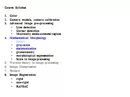
Color Camera models camera calibration Advanced image preprocessing Line detection Corner detection Maximally stable extremal regions Mathematical Morphology binary grayscale skeletonization. ef2010 11 Syllabus BT101E Introduction to Biotechnology wef 200 32004 Syllabus KURUKSHETRA UNIVERSITY KURUKSHETRA Established by the State Legislature Act XII of 19 56 A Grade NAAC Accredited DateSheet for BTech Engineering I Semester Exam ination c JAMESTOWN Thur 9 th October MINLATON Thur 30 th Oct KADINA Friday 14 th November Learn Safe Drive Safe 1 Day Course Full day course to learn and complete testing to obtain a Learners Permit Fee includes a GULYHU575265734757347KDQGERRN5735957347WUDLQ A PROGRAMME DISCIPLINE COURSE ECONOMICS COURSE CONTENTS Effective from the Academic Year 20112012 onwards DEPARTMENT OF ECONOMICS UNIVERSITY OF DELHI DELHI brPage 2br 2 Syllabus for BA Programme Economics Joint Fellows Symposium 2013. Dominik Wolff (IIT Fellow). Second Language Studies Program. What is SLA?. Second language acquisition (SLA) is the study of how second languages are learned and the factors that influence the process. . Course Design Intensive. June 2015. University of British Columbia, Centre for Teaching, Learning and Technology. Roselynn. . Verwoord. , MA. Isabeau Iqbal, PhD. This work is licensed under the Creative Commons Attribution-. SAMPLE COURSE LISTING June 1 5 - July 1 8 How to Read the Schedule of Classes Course Name Course Number Course Title Transferability Units Important Course Information Section Number Boxes denote s Jane West. Science Advisor 7-12. Secondary Education Directorate. Learning and Leadership Portfolio. Overview. Why . is the syllabus changing in NSW?. What. does the Science K-10 (incorporating Science and Technology K-6) syllabus look like?. Prepared by :. Asma. . Abas. Process syllabus : a syllabus which focuses on the means by which communicative skills will be brought about . (. Nunan. : 159 ). The aims center around the processes of learning rather than the product’’ (Bruner:1960). 1 1. you wish the Course Homepage, Course Admin, in the top hand corner. 2.On the next page, click Course Offering Information 3.In the list of options, you should see Active. Click the checkbox n as an . Effective . Communication Tool. Dr. Pam Brown, College of Education. Dr. Steve . Damron. , College of Agricultural Sciences and Natural Resources. 7 purposes of a syllabus. Sets the tone for the course. The best way to manage large projects is to scan the building and use the captured data to develop BIM models. This entire process is called as scan to BIM. So, BIM course training becomes more essential for construction or design engineers to understand its concept. NAAC BUSA 5 21 Fall 2018 The are subject to change. BUSA 5 21 – Project Management Fall 2018 INSTRUCTOR INFORMATION Instructor: Son Bui Office Location: BA 318 Office Hours: 10:00 am – Office Phone: The NIG Physics syllabus is divided into five sections which include;. Mechanics. Thermal Physics. Waves. Electricity and Magnetism. Atomic and Nuclear Physics. Electronics. NIG Syllabus . Khan Academy Resources.