PPT-EMS Wijeratne 1 , Charitha

Author : classyshadow | Published Date : 2020-08-27

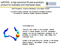
Pattiaratchi 1 and Roger Proctor 2 1 The UWA Oceans Institute The University of Western Australia 2 University of Tasmania Hobart Tasmania Australia ozROMS a

Presentation Embed Code

Download Presentation

Download Presentation The PPT/PDF document "EMS Wijeratne 1 , Charitha" is the property of its rightful owner. Permission is granted to download and print the materials on this website for personal, non-commercial use only, and to display it on your personal computer provided you do not modify the materials and that you retain all copyright notices contained in the materials. By downloading content from our website, you accept the terms of this agreement.

EMS Wijeratne 1 , Charitha: Transcript

Pattiaratchi 1 and Roger Proctor 2 1 The UWA Oceans Institute The University of Western Australia 2 University of Tasmania Hobart Tasmania Australia ozROMS a high resolution16 year reanalysis product for Australian and Indonesian Seas. MAY 17–23 EMS WEEK 2015EMS WEEK 2014 Welcometo the 2015 EMS Week Commemorative Guide ON BEHALF OFthe American College of Emergency Physicians (ACEP) and the National Association of Emergency Medi Per Dahlström Managing Authority. 20th October 2015 – Copenhagen, Denmark. Workflow . Input data. Partners. Project description. Work plan. Project budget. Attachments. Inputting budget data into the . Yakima County Emergency Medical Services. Candace Hamilton, EMS Manager. 2011. Topics. History. Purpose. Funding . Distribution. Frequently Asked Questions. History. History. 1985. Demand for EMS in Yakima County . . Let’s talk about . regeneration!. Christos Stefanou. MD, EDICM, PhD-cand. Assoc. Prof. Medicine. Internist, Intensivist.. Orlando, FL; Aug. 2015.. stefanouchristos@hotmail.com. Ockham Information Services LLC. 3 March 2011. History. National EMS Information System (NEMSIS.org). Version 3 data set, . de facto . standard. NEMSIS Sponsors. National Highway Transportation Safety Administration. Early work indicated ponies grazing high NSC pastures and having characteristics such as IR and obesity Were at greater risk of laminitis. . Resting . hyperinsulinaemia. predicts recurrence of laminitis in ponies on pasture. . (Building/Energy Management System). The future is now. Chris Peto, . 20.01.2015. Who Am I. System Software Engineer. , University of Maryland. Live in Dreieich, Germany. Resource Solutions. (since 1999). Healthcare is Transforming. Our nation’s healthcare system is transforming from a fee-for-service model . to . a patient-centered, . value- and . outcomes. -based model, known . as. “Healthcare 3.0” . Candace Hamilton, EMS Manager. 2011. Topics. History. Purpose. Funding . Distribution. Frequently Asked Questions. History. History. 1985. Demand for EMS in Yakima County . is. growing. System . identified . Objectives. Review the criteria for refusal of treatment and/or transport. Explain the use of the Quick Confusion Scale. Describe situations that require contact with Medical Control. Demonstrate the use of the revised PREMSS refusal form. March 9th, 2016. Program Description. H-33 EMS . Captain. : Paramedic Supervisor Role. SF DPH HOT . Outreach . Specialist: Care Coordination Role. Dispatched to 911 incidents. Special . c. alled . by other EMS Resources, clinics, case managers. A . Review and . Lessons Learned. . . Disclosure. Faculty: . Dr. Ian . Phelps – AHS Senior Medical Director EMS. Steen Pedersen – AHS EMS Provincial Director, Quality and Patient Safety. Welcome to Your EMS Certification Program Disclaimer All information for the forms presented by the Pennsylvania Department of Health (PA DOH), Bureau of Emergency Medical Services (BEMS), The Regional EMS Councils, and for the National Registry of Emergency Medical Technicians (NREMT) exams, at all EMS vs Car Asthma Outcomes by Mode of Transportation to a Pediatric ED Emily McFerren, MD Pediatric Emergency Medicine November 13, 2019 Outline Pediatric Asthma “EMS vs Car” study overview Practical applications

Download Document

Here is the link to download the presentation.
"EMS Wijeratne 1 , Charitha"The content belongs to its owner. You may download and print it for personal use, without modification, and keep all copyright notices. By downloading, you agree to these terms.