Confidence Intervals in Public Health tistics, sometimes they are inte - PDF document

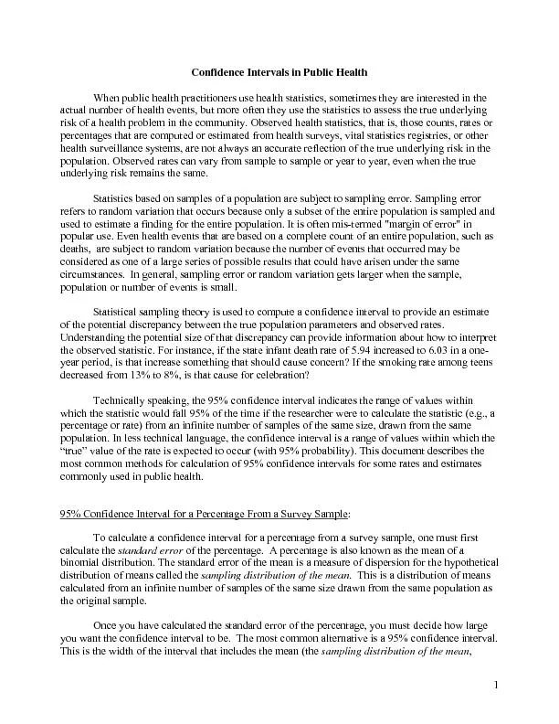
Confidence Intervals in Public Health tistics, sometimes they are interested in the actual number of health events, but risk of a health problem in the community. Observed health statistics,percentages that are computed or estimated from health surveys, vital statistics regihealth surveillance systems, are not always an accurpopulation. Observed rates can vary from sample to sample or year to year, even when the true underlying risk remains the same. Statistics based on samples of a population arerror. Sampling error refers to random variation that occurs because only a subset of the entire population is sampled and used to estimate a finding for the entire population. It is often mis-termed "margin of error" in popular use. Even health events that are based on a complete count deaths, are subject to random variation because the number of events that occurred may be considered as one of a large series of possible results that could have arisen under the same circumstances. In general, sampling error or random variation gets larger when the sample, population or number of events is small. Statistical sampling theory is used to compute a confidence interval to provide an estimate of the potential discrepancy between the true population parameters Understanding the potential size of that discrepancy can provide information about how to interpret year period, is that increase something that should cause concern? If the smoking rate among teens decreased from 13% to 8%, is that cause for celebration? which the statistic would fall 95% of the time if the researcher were to calculate the statistic (e.g., a percentage or rate) from an infinite number of samples of the same size, drawn from the same ). This document describes the most common methods for calculation of 95% confidence intervals for some rates and estimates 95% Confidence Interval for a Percentage From a Survey Sample To calculate a confidence interval for a percentage from a survey sample, one must first calculate the of the percentage. A percentage is also known as the mean of a binomial distribution. The standard error of the mean is a measure of dispersion for the hypothetical distribution of means called the sampling distribution of the meanribution of means calculated from an infinite number of samples of the same size drawn from the same population as the original sample. the percentage, you muterval to be. The most common alternThis is the width of the interval that includes the mean (the 1 mentioned above) 95% of the time. In a little plpercentage is the range of values within which the percentage will be found at least 95% of the time if you went back and got a different sample of the same size from the same population. Transforming the standard error into a 95% confidence interval is rather simple. has a shape that is almost identical to what is You need only multiply the standard error by the -score of the points in the normal distribution th -score is 1.96. A Z -score of 1.96 defines the 95% confidence interval. A Z -score of 1.65 defines a 90% confidence interval. For a simple random sample, the standard error = where: p is the rate, q is 1 minus the rate, and n is the sample size. Example: 13% of surveyed reconsisted of 500 persons in a simple random sample. The standard error = is a tool that is used in statistics to associate a statistic (e.g., a percentage, average, or other statistic) with its probability. When researchers talk about a measure being "statistically significant," they have used a to evaluate the probability of the statistic, and found that it would be improbable under ordinary conditions. In most cases, we can rely on measures such as rates, averages, and proportions as having an underlying normal , at least when the sample size is large enough. 2 Then the 95% confidence interval is: 1.96 * standard error = .13 + 1.96 * .015 = .13 + r limit of 10.1% and an upper limit of 15.9% The formula used above applies to a binomial distribution, which is thcomplimentary values (e.g., heads and tails, for a, such as an average, you’ll need to modify the equation. The a binomial distribution. If your man average, you must modify the formula, subsstandard error can also be calculated as the stasample size: Small Samples If the sample from which the percentage was calculated was rather small (according to central limit theorem we can define small as 29 or fewer) then the shape of the sampling distribution of the mean is not the same as the shape of the normal distribution. In this special case, the normal distribution.to those above but the t-score comes from a family of distributions that depeThe number of degrees of freedom is defined as “n-1” where “n” is the size of the sample. For a sample offreedom is equal to 29. So, for a 95% confidence interval, you must use the t-29 degrees of freedom. That particular t-score is 2.045 (see Appendix 1.). So you would multiply If our sample were a different size, say 20, then the degrees of freedom would be 19, which is associated with a wider as our sample size is reduced. This reflects the uncertainty in our estimate of the variance in rval with 9 degrees of freedom the -score is 2.262. Table 1. lists the t sizes of confidence interval. For a 95% ribution that excludes the most extreme 5% of the distributio Student's t-distribution, downloaded on 2/13/09 from http://en.wikipedia.org/wiki/File:Student_densite_best.JPG 3 Distribution at Varying Degrees of Freedom (k) Appendix 1 lists the t-scores for specific degrees of freedom and sizes of confidence that defines the points on the distribution that excludes the most extreme 5% of If the survey sampled all or most of the mepopulation correction factor will improve (decr, where is the sampling fraction ion. The sampling fraction is simply the proportion of the population that was included in the sample. The standard error of the mean for a binomial distribution for a finite sample percentage When the Percentage is Close to 0% or 100% When the percentage is close to 0% or 100%, the formulas given above can result in illogical results - confidence limits that fall below 0% or above 100%. A special formula is used to calculate asymmetric confidence limits in these cases. Because survey estimates can be small percentages, the confidence intervals for the survlogit transformations. Logit transformations yield asymmetric interval boundaries that are more ba 4 standard symmetric confidence intervals for small proportions. The method used is as follows: (1) Perform a logit transformation of the original percentage estimate: f = log(p)-log(1-p) p = the percentage estimate f = the logit transforma(2) Transform the standard error of the percentage to a standard error of the it’s logit transformation: se(f) = se(p)/(p*(1-p)) se = standard error e logit transformation Lf = f - t(alpha/2, df)*se Uf = f + t(alpha/2, df)*se Lf = lower confidence bound of f Uf = upper confidence bound of f t(alpha/2, df) = the value of the t-score corrdegrees of freedom (degrees of freedom is defined as “n-1” where “n” is the sample size). (4) Finally, perform inverse logit transformations to get Lp = exp(Lf)/(1+exp(Lf)) Up = exp(Uf)/(1+exp(Uf)) Lp = lower confidence bound of p Complex Sample Designs The above formulas assume that the survey sample was a survey used a complex sample design (such as sampling from various geographic regions), special techniques must be used to calculate the standard error of the mean. Those techniques are accomplished using statistical software such as When the Rate is Equal to 0 zero, using the above calculation will yield a ect. A simple method you can use to estimate the 5 zero is to assume the number of cases in the numerator of your rate is “3,” then calculate th95% Confidence Intervals for Rare Events: randomly across time, the normal distribution no distribution is used to model rare events that occur across time, such as the "100 year flood." It is used to calculate confidence intervals for rare health events, such as infant mortality or cancer.symmetric about its mean and so the associated confidence intervals will not be symmetric (the upper limit is farther from the estimate than is the lower limit). The Poisson distribution does, however, assume the shape of a normal distribution when there are 20 or more events in the numerator. Sobution for rare events (when the number of events is less than 20), but we can use the normal distribution when the number of events is 20 or more. In Appendix 2 you will find lower and upper confidence factors for use in calculating a 95% number of events, from 1 to 20. To calculate the confidence interval, multiply the estimated rate by the confidence factor associated with the number Lilienfeld, DE and Stolley, PD Foundations of Epidemiology (3rd Ed.). Oxford University Press, 1994. “In probability theory and statistics, the Poisson distribution is a discrete probability distribution that expresses the probability of a number of events occurring in a fixed period of time if these events occur with a known average rate and independently of the time since the last event.” , downloaded on 2/13/09 from http://en.wikipedia.org/wiki/Poisson_distribution . 6 For example, in a given geographic area, therinfant deaths. The infant mortality rate in[(7/722)*1,000]. The lower and upper confidence limitslimits of the confidence interval, respectively. The lower limit of the confidence interval = 9.7*.4021 = 3.90, and the upper limit = 9.7*2.0604 = 19.99, for a rate of 9.7 and a 95% confidence interval from 3.90 to 19.99. If this same rate halimit would be 9.7*.8136, and the upper limit 9.7*1.2163 for an estimate of 9.7 with a confidence interval from 7.89 to 11.80. This interval is much smaller due to the greater number ofIn the Utah IBIS-PH query system, startiinterval), and the two parameters associated with the distribution function: the mean and the variance. In the case of the crude rate, where the variance and mean are equal, this is the special case of the gamma family of distributi When comparing across geographic areas, some method of age adjusting is typically used to control for area-to-area differences in health eventsarea populations. For example, an area that has an older population will have higher crude (not age-are the same as those of other areas. One might incorrectly attribute the high cancer rates to some justed rates control for agcomparability of rates across areas. Direct standardization adjusts the age-specific rates observed in the small area to the age distribution of a The directly age-adjusted death rate is a weighted average of the age-specific death rates where the Directly age-adjusted death rate (DAADR) = Wsi * Di/ Pi = = the weight for the i = number of deaths (or other event) Lilienfeld, DE and Stolley, PD (1994) 7 ) = var(DThe variance of a directly age-adjusted death rate can then be computed as follows: se(DAADR) = square root (var(DAADR)) = the weight for the i) = the variance of the age-specific death rate in the i = number of deaths (or other event)se(DAADR) = standard error of th The age-adjusted death rate is a linear combination of independent Poisson random variables and therefore is not a Poisson random variable itself. It can be plfamily of gamma distributions of which the Poisson is a member. Statistical packages such as SAS have a function to calculate factors that may be applied to age-adjusted death rates to calculate 95-ese factors are derived from a In the IBIS-PH query system, starting in Maparameters associated with the distribution function: the mean and the variance. In the case of the age-adjusted rate, the variance and mean are not accounted for in the calculation of the confidence factors used to compute the gamma confidence intervals for age- Gamma intervals perform well even when the number in any specific age-adjustment age group cell is small. Indirectly Age-Adjusted Rates The direct method can present problems when population sizes are particularly small. specific rates, and for small areas these age-specific rates may be based on one or two Anderson RN, Rosenberg HM, Age Standardization of Death Rates: Implementation of the Year 2000 Standard. National vital statistics reports; vol 47 no.3. Hyattsville, Maryland: National Center for Health Statistics. 1998 Fay MP, Feuer EF, Confidence Intervals for Directly Standardized Rates: A Method based on the Gamma Distribution. Statistics in medicine, vol 16, 791-801 (1997) 8 there are fewer than 20 (some say 25) cases in thIndirectly standardized rates are based on the Standardized Mortality Ratio (SMR) and the death or disease rate (ISR) can be computed as: observed deaths/disease in the small area = D = D expected deaths/disease in the small area e SMR = observed deaths in the small area/expected deaths in the small area D = observed number of deaths in the small area ) = expected number of deaths in small area e group i of the small area ts that follow a Poisswhich the ratio of events to total population is small () the sample size is large, the following two methods can be used to calculate confidence interval (Kahn & Sempos, 1989)(1) When the number of events 20: CIISR = + 1.96 (SMR/e) * Rs * K Lilienfeld & Stolley (1994) Rothman, Kenneth J. and Greenland, Sander (1998) Modern Epidemiology (2nd Ed.). Philadelphia, PA: Lippincott. Harold A. Kahn and Christopher T. Sempos (1989) Statistical Methods in Epidemiology . New York: Oxford University Press. 9 SMR = observed deaths in the small area/expected deaths in the small area e = expected deaths in the small area = (2) When the number of events = (Lower limit for parameter estimate from Poisson table/e)) * R = (Upper limit for parameter estimate from Poisson table/e)) * RLL is the lower confidence interval limit, and UL is the upper confidence interval limit. Document created Public Health Assessment, Utah Department of Health Images of sampling Lois M. Haggard, Community Health Assessment Program, New Mexico Department of Health Asymmetric confidence intervals for percentages c Disease Bureau, Utah Department of Health, Kathryn Marti, Brian Paoli, Office of Public Health Assessment, Utah Department binomial distributions Lois M. Haggard, Community Health Assessment Program, New Mexico Department of Health Confidence Intervals for Rare Events’ and ‘Directly Age-adjusted Rates’ re: calculate confidence intervals for rare events. Kathryn Marti, Brian Paoli, Office of Public Health Assessment, Utah Department of Health 10 Appendix 1. Upper critical values of Student's t distribution with degrees of freedom 1 6.314 12.706 31.821 318.313 2 1.886 22.327 3 1.638 10.215 4 1.533 5 1.476 6 1.440 7 1.415 8 1.397 9 1.383 10 1.372 11 1.363 12 1.356 13 1.350 14 1.345 15 1.341 16 1.337 17 1.333 18 1.330 19 1.328 20 1.325 21 1.323 22 1.321 23 1.319 24 1.318 25 1.316 26 1.315 27 1.314 28 1.313 29 1.311 30 1.310 11 Appendix 2. 95% Confidence Interval Factors for Poisson-Distributed Events 95% Confidence Interval, Lower Limit Factor 95% Confidence Interval, Upper Limit Factor 0 3.7000 1 5.5716 2 3.6123 3 2.9224 4 2.5604 5 2.3337 6 2.1766 7 2.0604 8 1.9704 9 1.8983 10 1.8390 11 1.7893 12 1.7468 13 1.7100 14 1.6778 15 1.6493 16 1.6239 17 1.6011 18 1.5804 19 1.5616 20 1.5444