PDF-Mechanisms of Categorization in InfancyIn Infancy (ex-Infant Behaviour

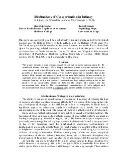
Mechanisms of Categorization in InfancyThe ability to categorize underlies much of cognition It is a way of reducing the loadon memory and other cognitive processes Roch 1975 Because of its funda. 46 Breakdown mechanisms in BJTs The breakdown mechanisms of BJTs are similar to that of p n junctions Since the base collect or junction is reversed biased it is this junction where breakdown typically occurs Jus Categorization. . With. . Bags. of . Keypoints. Original . Authors. :. G.. . Csurka. , C.R. Dance, L. Fan, . J. . Willamowski. , C. Bray. ECCV Workshop on . Statistical. Learning in Computer – 2004. Talk Overview. Background. : Understand infant cognitive development. The Problem of Tool Use. : . What is required. What develops . Mechanisms of Development: . . Behavioural schemas (Six mechanisms). Physical Growth. The brain. Infant states. Nutrition. Motor development. Sensory and perceptual development. Piaget’s theory. Learning. Intelligence. Language. Emotional developmt.. Temperament. Personality. Tanja Svarre & Marianne Lykke, Aalborg University, DK. ISKO . conference. , 8th of . July. , 2013.. Agenda. Background of the . study. Theoretical. . framework. Research . methods. Results. Summary and . Concepts and Categorization. Concepts . allow for efficient . categorization. But, how are . concepts represented. ?. What “defines” an object?. Primary qualities. Secondary . qualities. How do we decide ‘object X’ belongs. Lesson 2. Starter one. From last lesson. What should an evaluation include? . Write on my board. Activity- Neural pub quiz- Group work. Create . four . questions based on homework on neural mechanisms and a . Lesson three. Neural mechanisms. How does the research support the N.M theory?. Crockett et al (2008). carried out a repeated measures experiment on 20 participants. . In . both conditions the participants had fasted and were given a protein drink in the morning before taking part in the study. The difference in the drink was the difference in the conditions: one drink contained tryptophan, which the body needs to make serotonin; the other drink did not contain it. On both days that the study took place participants played the ultimatum game. In this game one player poses a way to split a sum of money with a partner. In the condition where the participants had had the drink that did not contain tryptophan (so their serotonin levels were low) they showed increased aggression toward offers they perceived to be unfair.. Security Categorization of Information and Information Systems. Purpose: . To establish protection profiles and assign control element settings for each category of data for which an Agency is responsible. Security Organization is the basis for identifying an initial baseline set of security controls for the information and information systems. . Do Now:. How does Hamilton want to handle paying the debt . of America?. US Infancy. The first few decades of American history. US INFANCY – infant – baby. US is a “baby” country. Weak/fragile. Infancy and Childhood. Module 11. Maturation. : Biological . growth . processes that enable orderly changes in behavior. Relatively uninfluenced by experience. Severe . deprivation or abuse can slow development, yet genetic growth patterns are inborn. Applications:. Web pages . Recommending pages. Yahoo-like classification hierarchies. Categorizing bookmarks. Newsgroup Messages /News Feeds / Micro-blog Posts. Recommending messages, posts, tweets, etc.. Abstract Infant and child development is a complex interaction between environmental, biological, social, cultural, and familial factors influenced by neighborhood and community context and operating from preconception, through gestation, infancy, and childhood. T. OHKI, K. WATANABE, T. NEGORO, K. ASO, Y. HAGA, K. KASAI, M. KIT0 & N. MAEDA Department of Pediatrics, Nagoya University School of Medicine, Nagoya, Japan Changes in seizure type of severe myoclon