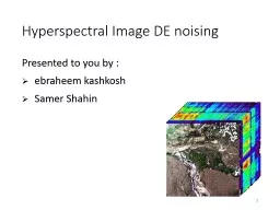
Hyperspectral Image DE noising - PowerPoint Presentation

Slide1

Hyperspectral Image DE noising

Presented to you by :ebraheem kashkosh Samer Shahin

1

Slide2

A Technique For Removing Second-Order Light Effects From Hyperspectral Imaging Data

2

Slide3

schedule

quick introReview Second-Order Light problem

Experimental way to solve+results DISCUSSION

3

Slide4

HICO–Hyperspectral Imager for coastal Oceans

The Hyperspectral imager for the Coastal Ocean (HICO) currently onboard the ISS .it is a new sensor designed specifically for the studies of turbid coastal water and large island lakes and rivers .

The HICO covers the wavelength range between 0.35 and 1.08 µm with a spectral resolution of 5.7nm and spatial resolution of 90m.

4

Slide5

Bad News 9

It was originally planned that a second-order blocking filter would be placed close to the focal plane array (FPA) of HICO, but mechanical mounting problems were encountered

And many sensors like HICO ,Airborne Imaging Spectromete, …built without a blocking filter to eliminate the second-order light effects.

5

Slide6

The HICO - Problem

the HICO sensor is not equipped with second-order blocking filter .

as a result , the second-order light in the wavelength interval between 0.35 and 0.54 μm falls in the same pixels as the first-order light in the 0.7–1.08-μm wavelength interval.

In order to have accurate radiometric calibration of the near-IR channels , the second-order light contribution needs to be removed .

6

Slide7

Second-order light

it follows from the theory of diffraction gratings that different diffraction orders overlap, i.e. a photon with

wavelength in the m-th order will be diffracted at the same direction as a photon with wavelength

from the m+1-st order and thus both will be recorded at the same pixel on the detector.

For diffraction gratings the relation between

and

is simple,

= [(m + 1)

]/m

 

7

Slide8

Second order-light cont.

Focal plane

1

st

order light

2

nd

order light

lens

1

st

&2

nd

order light falls on the same pixel

8

Slide9

Bad news

9

Slide10

Observations

Through analysis of Hyperspectral imaging data collected with the Airborne Visible/infrared Imaging Spectrometer (AVIRIS ) ,found that :

In deep waters For wavelength greater than about 0.75 µm the transmittances are close to zero while the transmittance at 0.55 µm in the visible is as large as 90%

Note : AVIRIS is equipped with several order-separation filters . Thus it is

free

of the second-order light effects

10

Slide11

Observations from AVIRIS DATA

Fig. 1(a) shows a true-color AVIRIS red–green–blue (RGB) image (red: 0.66 μm; green: 0.55 μm; blue: 0.47 μm) acquired over French Frigate Shoals in Hawaiian waters in April of 2000. Underwater features, such as coral reefs (spot in light green color) and shallow water (in light blue color), are clearly seen.

Fig. 1(b) shows a 1.0-μm single-channel image of the same scene. Underwater coral reef features are no longer seen in this image because of strong liquid water absorption in the near-IR spectral region.

11

Slide12

Experimental way to solve

2(a) the liquid water absorption coefficient in the range of 0.3–1.1 μm.

2(b)shows the calculated transmittance spectrum for light passing through a liquid water layer with a thickness of 4 m

we expect that the underwater objects 2 m below the air–water interface will be seen in visible channel images but not in images of near-IR channels above 0.75 μm.

12

Slide13

Experimental way to solve

From fig 1(b) we realized that the underwater features in these images resulted from the second-order light of visible channels.

13

Slide14

midway island

14

Slide15

Experimental way to solve+result

15

Slide16

Experimental way to solve

To develop the method, we extract a pair of spectra over shallow water S(λ) and nearby deep water D(λ)

16

Slide17

S(λ) − p(λ)S(λ/2) = D(λ) − p(λ)D(λ/2)

S(λ) is the signal rom the shallow- water area at λD(λ) is the signal from the deepwater area at λp(λ) is the empirical scaling factor for correcting the

second-order light effectp(λ) S(λ/2) on the left side of (1) is the second-order signal at the near-IR wavelength λ contributed by the signal at λ/2 for the shallow-water spectrum

For λ = 0.9 to 1.1 transmittance spectrum for light is zero

For λ/2 = 0.45 to 0.55 transmittance spectrum for light is about 90%

17

Slide18

** p(λ) = [S(λ) − D(λ)] / [S(λ/2) − D(λ/2)]

In order to generate p(λ) for the second-order light corrections to all HICO data, we selected a number of pairs ofshallow-water and nearby deepwater spectra. We calculatedan empirical curve for each pair of spectra using **

18

Slide19

Empirical scaling factors as a function of wavelength for second-order light corrections over different locations.

The black line shows the averaged values of all the locations

19

Slide20

After generating the scale factor p(λ), we make the correction for HICO data sets on a pixel-by-pixel basis.

The equation to correct the data isC(λ) = f (λ) − p(λ) ∗ f (λ/2)

20

Slide21

C(λ) = f (λ) − p(λ) ∗ f (λ/2)

f (λ) is the signal at λp(λ) is the correcting factor p(λ) ∗ f (λ/2) is the second order contributionC(λ) is the signal after the second-order

correction.

21

Slide22

22

Slide23

It is noted that the two small islands, the circle around the edge of the atoll, and clouds are still present.

The circle is most likely resulted from the scattering of solar radiation by foams from breaking waves, and it is not due to the second-order effect of visible light.

23

Slide24

24

Slide25

result

25

Slide26

The two images used the same color bar

DNs are approximately in the range between 70 and 140 in shallow-water areas and about 40–60 in deepwater areas before the correction

After the correction, the DNs over both the shallow waters and deep waters are reduced as shown it is seen quantitatively the dramatic reduction of unwanted DNs after the removal of the second-order light effect.

26

Slide27

DISCUSSION

27

Slide28

Ideally, there would be no spread in the curves shown in Fig. 4. To explain the existence of the spread, we first examine in more detail the assumption that no light comes from below the water surface at near-IR wavelengths.

28

Slide29

Inspection of Fig. 2(a) shows that the 1/e absorption path of water at this wavelength is about 15 cm.

Thus, if the water column contains a significant amount of scattering material within a quarter meter or so of the surface, the assumption that no light is returned from below the surface may not be strictly valid. This contribution to the signal in (1) would cause an error in the calculation of p(λ) using (2)

29

Slide30

30

Slide31

As noted in Section III, the shallow-water and deep water comparison points were chosen just inside and just outside of the coral reefs.

Atmospheric path radiance normally changes very slightly over a distance of a few kilometers, but it is possible that the atmosphere, particularly the near-surface atmosphere, is sufficiently different between the two points that the assumption of the constancy of atmospheric path radiance is not strictly valid.

31

Slide32

Part 2

Recovering Junk bands

32

Slide33

Introduction

In modern Hyperspectral imaging systems ,many of the spectral bands have high SNR, but a significant number of bands (up to 20 percent) are extremely noisy due to atmospheric effects.Denoising these bands lead to higher classification performance , especially if the recovered bands contain spectral features useful for discriminating between classes.

33

Slide34

Recovering Junk Bands using Wavelets and Sparse Approximation

Two algorithms are proposed :

Denoising an entire data cube ( the HS-images)Recovers user designated junk bandsBoth algorithms utilize a combination of wavelet and

sparse approximation techniques .

But we will only consider the second one in this presentation

34

Slide35

Visual aid

Good bands

Bad bands

35

Slide36

Wavelets (Reminder)

Taken from last year "Image processing course" , with our lecturer Prof Hagit

36

Slide37

Wavlets cont.

Motivation:-Wavelet domain – tells you “what” is happening and “where” - a local description of image

37

Slide38

Wavelets – How does it work ?!!

When applying a 2d DWT on an image we get : vertical , horizontal & diagonal magnitudes of the image.

a down sampled (by 2) image of the original image.

down sampled

horizontal coefficients

diagonal coefficients

Vertical coefficients

38

Slide39

We repeat the process on the down sampled image until we reach the desired level.

39

Slide40

Construction

:

Apply the 4 filters on the frequency domain of the image :

The vertical

the horizontal

the diagonal

the low pass filter

Down sample the image

Repeat until you reach the desired result

Reconstruction

:

Sum up all the current level

Expand by 2

Repeat

Wavelet Pyramid in Frequency domain

40

Slide41

41

Slide42

42

Slide43

Sparsity of wavelet representations

Applying a 2-D DWT to an image corrupted by additive white Gaussian noise (AWGN) results in a sparse representation. in terms of magnitude : small number of large coefficients,(those containing signal + noise ) And majority are small ( noise only) .

Intuition : denoising by zeroing out the noise coefficients while retaining signal coefficients;

*Note : DWT =

Discrete Wavelet Transform

43

Slide44

definitions

() and

() are the 2-D DWT and 2-D inverse DWT operators , respectively .

I = N x M noisy image.

(I) is a sparse matrix .

vec(

(I) ) : arrange the matrix

into a single column .

Let

be a set of high SNR band

images

(

))

* note :

is a sparse vector

 

44

Slide45

Sparse approximation

Sparse approximation Goal is to find a sparse vector x of unknowns such that y = Axy ∈

, A ∈

,

x ∈

, and M <N

Y and A are given , x is unknown

we will enforce sparsity on x by minimizing the ||x||

0 (number of nonzero element of X)

 

45

Slide46

Sparse approximation

The above optimization problem

is NP-Complete.

So Let us relax the problem and minimize the

l1 norm

of

x rather than its number of nonzero elements

Solved in linear time .

46

Slide47

Sparse approximation

Noisy image case : y = Ax+n , n∈ R^N (noise).Due to the noise, it is unlikely that a sparse x exists

such that Ax exactly equals y. A more practical solution is to find a sparse x that approximately

solves the noisy system.

This is done by the next formula ..

47

Slide48

Sparse approximation

As the regularization parameter, λ, is increased from zero to one, the algorithm yields sparser and sparser solutions and the residual error increases. Thus, λ is a control parameter that trades off sparsity versus residual error.

Keeps the residual error down

Enforces sparsity on x

48

Slide49

Sparse approximation

Now suppose we have a set of noisy vectors:

i = 1, . . . , T . Letting Y = [

, . . . ,

] and X = [

, . . . ,

],

we generalize (1) into a program that finds an

X that approximately

solves

Y = AX, with the constraint that each column of X (i.e.,

each of the

xi) have a similar sparsity profile. We pose the problem

as follows:

 

49

Slide50

Frobenius norm

The Frobenius norm  is matrix norm of an MxN matrix A defined as the square root of the sum of the absolute squares of its elements.

Example:

 

50

Slide51

The fiendish

 

 s

51

Slide52

Back to the formula

Y and A are given .We need to find X .

λ is a constant chosen by experimentation . This problem is solved by using SeDuMi toolbox .

Keeps the residual error down

Enforces sparsity on every

in X

 

52

Slide53

Denoising algorithm

Finally

53

Slide54

Denoising algorithm

we explained that band images in a high SNR data cube are correlated, and thus their wavelet coefficients have similar sparsity patterns.

Let

be a set of noisy band images.

There is a true (non-noisy) image within each

, each of which has a similar sparse representation in the wavelet

domain.

Our algorithm recovers the clean images within each image by imposing the same sparsity pattern on the wavelet coefficients of each

 

54

Slide55

Denoising algorithm

Perform a J-level 2-D DWT on each

and get

.

Let D =[

…….,

] and

= [

,….. ,

]

For each I, find a

that is close to

in an

norm sense , while enforcing the sparsity on every

to be similar .

Thus we get to the problem of :

-find a

that is close to D in the Frobenius-norm

sense and whose columns have similar sparsity profiles.

This is done by

Sparse approximation

formula

 

55

Slide56

Denoising algorithm

4. This is done by solving the Sparse approximationformula :

5. Each column of

contains the denoised detail coefficients of

image

. Extract the columns of

to yield {

}. Reform a set

of 2-D wavelet coefficients using the

’s scaling coefficients and

the denoised detail coefficients ˆ

. Perform a 2-D IDWT on this

data, yielding

, a denoised version of

 

56

Slide57

Denoising algorithm –visual aid

D =

2d-DWT coefficient of

 

2d-DWT coefficient of

 

2d-DWT coefficient of

 

…

…

is a set of noisy band images

 

57

Slide58

Denoising algorithm –visual aid

First term :

-

 

…

…

-

 

-

 

F

(1-

λ

)

58

Slide59

Denoising algorithm –visual aid

Second term :

 

of every row of D^

 

λ

λ

Apply

norm on every row of

 

R

contains coefficient j of every

 

Apply

norm

 

This is a vec not a matrix

59

Slide60

Denoising algorithm

The algorithm we showed denoises a set of bad bands in an image by enforcing their 2d-dwt (Discrete Wavelet Transform ) to have a similar sparsity profile.so far we didn’t use the data in the good bands of the image . And next we will show how to recover the bad bands by enforcing their 2d-dwt to have a similar sparsity profile as the good bands .

60

Slide61

Junk band recovery algorithm

Let

and

be a set of

user designated

good band and junk bands.

Contains a bands with high SNR

Contains a bands with Low SNR.

Let

=

be the averaging K good bands .

Let

Note : this vector have an obvious sparsity profile since it’s the average of a high SNR bands ( low noise )

 

61

Slide62

Junk band recovery algorithm cont.

Compute

By performing a 2-d Dwt on each OF THE

.

. D =[

…….,

]

 

62

Slide63

Junk band recovery algorithm cont.

Find a matrix

with two properties :Column should be close to those of D

Each column of

should have a sparsity profile similar to

We find such matrix by solving the following problem :

Were G=[D,

] . Append

to the matrix D.

,

}

 

63

Slide64

Junk band recovery algorithm cont.

Next step :Extract

from the resulting

.

 

=

 

 

 

……………...

………………………….......

……………...

……………...

……………...

64

Slide65

Junk band recovery algorithm cont.

Finally reconstruct the images :for each I (band) recover a denoised version of junk band

by doing a 2-D IDWT on

’s original scaling coefficients and its denoised detail coefficients

 

65

Slide66

Summary

First we defined noisy bands and good bands .Then we applied 2d discreet wavelet transformation on the bands .

Using the sparsity approximation method we enforced the sparsity profile of the bad bands to be like the sparsity profile of the good bands.We then applied inverse discreet wavelet transformation to on the results to obtain the denoised bandsEnjoy

66

Slide67

Results and experiments

67

Slide68

Comparison to other methods

First Experiment :Given a data cube ( meaning a Hyperspectral image) that contains 200 bands

Add a known Standard deviation

(noise ) to first 10 bands .

Run our algorithm (using specified values for

.

run a standard Donoho-Johnstone wavelet thresholding techniques

Compute the MSE of the denoised bands .

Compare results with our algorithm

 

68

Slide69

Comparison to other methods cont.

The MSE / 10^4 between each denoised band image and the corresponding original band image.

Note : the MSE between the noisy band and the originale one is 6.25*10^4 and 25*10^4For

 

Our algorithm

The Other algorithms

69

Slide70

Comparison cont.

70

Slide71

Second Experiment

Second experiment testing real data :Given a Hyperspectral image with good and bad bands .We identify bands 104 through 113 as junk bands

114 through 135 good bandsRun our algorithm Get results .

71

Slide72

Second Experiment results

72

Slide73

The End ..hurray

73

Slide74

Reference

Second order light removal: http://hico.coas.oregonstate.edu/publications/Li_IEEE_Transactions_2012.pdf

Diffraction grating :http://www.not.iac.es/instruments/alfosc/AN.2007.328.9.948.pdf

Recovering junk bands using wavelets :

http://www.rle.mit.edu/stir/documents/ZelinskiG_IGARSS2006.pdf

.

Wavelets explanation

Image processing course with professor hagit (2015)

74

Slide75

Reference

Second order light removal videos: https://www.youtube.com/watch?v=OHTpxHxuAhYhttps://www.youtube.com/watch?v=sCrfqIWMDzI

https://www.youtube.com/watch?v=Gw-Ry0xDtfs

75

Slide76

Backup slides

76

Slide77

SNR-signal to noise ratio

traditionally, SNR has been defined as the ratio of the average signal value

  to the 

standard deviation

  

of the background:

 

77

Slide78

The haar wavelet

To calculate the Haar transform of an 1d array of n samples:Treat the array as n/2 pairs called (a, b)

Calculate (a + b) / sqrt(2) for each pair, these values will be the first half of the output array.

Calculate 

(a - b) / sqrt(2)

 for each pair, these values will be the second half.

Repeat the process on the first half of the array.

(the array length should be a power of two)

78