/
Track Short Course: Track Introduction and Commands Track Short Course: Track Introduction and Commands

Track Short Course: Track Introduction and Commands - PowerPoint Presentation

ellena-manuel
ellena-manuel . @ellena-manuel
Follow
483 views
Uploaded On 2015-11-28

Track Short Course: Track Introduction and Commands - PPT Presentation

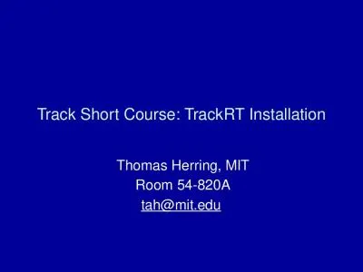
Lecture 01 Thomas Herring MIT Room 54820A tahmitedu Schedule Lectures 9001030 and 11001230 Tutorial sessions 13301700 Tuesday Cover track the postprocessing program Wednesday Cover ID: 207545

trackshortcourse file l01 2011 file trackshortcourse 2011 l01 track data site sites seminar time anu ionospheric delay ambiguity command

Share:

Link:

Embed:

Download Presentation from below link

Download Presentation The PPT/PDF document "Track Short Course: Track Introduction a..." is the property of its rightful owner. Permission is granted to download and print the materials on this web site for personal, non-commercial use only, and to display it on your personal computer provided you do not modify the materials and that you retain all copyright notices contained in the materials. By downloading content from our website, you accept the terms of this agreement.


Presentation Transcript

Slide1

Track Short Course: Track Introduction and CommandsLecture 01

Thomas Herring, MIT

Room 54-820A

tah@mit.edu

Slide2

ScheduleLectures 9:00-10:30 and 11:00-12:30;

Tutorial sessions 13:30-17:00

Tuesday: Cover track, the post-processing program

Wednesday: Cover trackRT, real-time processing and trackRTr the post-processing version of trackRT (used for analysis and tuning of trackRT).

04/26/2011

TrackShortCourse L01

2Slide3

04/26/2011TrackShortCourse L01

3

Kinematic GPS

The style of GPS data collection and processing suggests that one or more GPS stations is moving (e.g., car, aircraft)

To obtain good results for positioning as a function of time it helps if the ambiguities can be fixed to integer values. Although with the “back smooth” option in track this is nit so critical.

Program

track

is the MIT implementation of this style of processing

. The real time version is

trackRT

Unlike many programs of this type, track pre-reads all data before processing. (This approach has its pros and cons)Slide4

04/26/2011TrackShortCourse L01

4

General aspects

The success of kinematic processing depends on separation of sites

If there are one or more static base stations and the moving receivers are positioned relative to these.

For separations < 10 km, usually easy10>100 km more difficult but often successful

>100 km very mixed results depending on quality of data collected.

Slide5

04/26/2011TrackShortCourse L01

5

Issues with length

As site separation increases, the differential ionospheric delays increases, atmospheric delay differences also increase

For short baselines (<2-3 km), ionospheric delay can be treated as ~zero and L1 and L2 ambiguities resolved separately. Positioning can use L1 and L2 separately (less random noise).

For longer baselines this is no longer true and track uses the MW-WL to resolve L1-

L2 cyclesSlide6

04/26/2011TrackShortCourse L01

6

Track features

Track uses the Melbourne-Wubena Wide Lane to resolve L1-L2 and then a combination of techniques to determine L1 and L2 cycles separately.

“Bias flags” are added at times of cycle slips and the ambiguity resolution tries to resolve these to integer values.

Track uses floating point estimate with LC, MW-WL and ionospheric delay constraints to determine the integer biases and the reliability with which they are determined.

Kalman filter smoothing can be used. (Non-resolved ambiguity parameters are constant, and atmospheric delays are consistent with process noise). When atmospheric delays are estimated, the smoothing option should always be used.Slide7

04/26/2011TrackShortCourse L01

7

Ambiguity resolution

Algorithm is “relative-rank” approach. Chi-squared increment of making L1 and L2 ambiguities integer values for the best choice and next best are compared. If best has much smaller chi-squared impact, then ambiguity is fixed to integer values.

Test is on inverse-ratio of chi-squared increments (i.e., Large relative rank (RR) is good).

Chi-squared computed from:

Match of LC combination to estimated value (LC)

Match to MW-WL average value (WL)

Closeness of ionospheric delay to zero (less weight on longer baselines) (LG)

Relative weights of LC, WL and LG can be set.

Estimates are iterated until no more ambiguities can be resolved.Slide8

04/26/2011TrackShortCourse L01

8

Basic GPS phase and range equations

Basic equations show the relationship between pseudorange and phase measurementsSlide9

04/26/2011TrackShortCourse L01

9

L1-L2 and Melbourne-Wubena Wide Lane

The difference between L1 and L2 phase with the L2 phase scaled to the L1 wavelength is often called simply the widelane and used to detect cycle slips. However it is effected fluctuations in the ionospheric delay which in delay is inversely proportional to frequency squared.

The lower frequency L2 has a larger contribution than the higher frequency L1

The MW-WL removes both the effects on the ionospheric delay and changes in range by using the range measurements to estimate the difference in phase between L1 and L2Slide10

MW-WL Characteristics

In one-way form as shown the MW-WL does not need to be an integer or constant

Slope in one-way is common, but notice that both satellites show the same slope.

If same satellite-pair difference from another station (especially when same brand receiver and antenna) are subtracted from these results then would be an integer (even at this one station, difference is close to integer)The MW-WL tells you the difference between the L1 and L2 cycles. To get the individual cycles at L1 and L2 we need another technique.There is a formula that gives L1+L2 cycles but it has 10 times the noise of the range data (

f/f) and generally is not used.

04/26/2011

TrackShortCourse L01

10Slide11

04/26/2011TrackShortCourse L01

11

Melbourne-Wubena Wide Lane (MW-WL)

Equation for the MW-WL. The term Rf/c are the range in cycles (notice the sum due to change of sign ionospheric delay)

The

f/

f term for GPS is ~0.124 which means range noise is reduced by a about a factor of ten.

The ML-WL should be integer (within noise) when data from different sites and satellites (double differences) are used.

However, receiver/satellite dependent biases need to be accounted for (and kept up to date).Slide12

04/26/2011TrackShortCourse L01

12

Example MW-WL PRN 07 and PRN 28)Slide13

EX-WL Extra-Wide-laneThe other measure of the difference in cycles between L1 and L2 used by track is the EX-WL (Extra

Widelane

).

This measure is independent of geometry but is affected by the ionospheric delays. On short separations this measure is often more robust than the MW-WL.04/26/2011

TrackShortCourse L01

13Slide14

04/26/2011TrackShortCourse L01

14

Basic

Inputs for track.

Track runs using a command file

The base inputs needed are:

Obs_file

specifies names of

rinex

data files. Sites can be K kinematic or F fixed

Nav_file

orbit file either broadcast ephemeris file or sp3 file

Mode air/short/long -- Mode command is not strictly needed but it sets defaults for variety of

situations

Normally

back_type

smooth would also be specified.

Normally start with just these commands and see how the run looks and based on this output start tuning track. Slide15

04/26/2011TrackShortCourse L01

15

Basic use

Recommended to start with above commands and see how the solution looks

Usage: track -f track.cmd >&! track.out

Basic quality checks: grep RMS of output file

Kinematic site rovr appears dynamic Coordinate RMS XYZ 283.44 662.53 859.17 m.

For 2067 Double differences: Average RMS 17.85 mm

Check track.sum file for ambiguity status and RMS scatter of residuals.Slide16

04/26/2011TrackShortCourse L01

16

Track command line

% track -

f

<command file> -a <ambiguity file> -d

<day> -

w

<week> -

s

<S01> <S02> .. <S10>

where <command file> is a required file containing a list of

commands

to control the program (see below)

<ambiguity file> is an optional file containing a

modified set

of integer bias parameters and settings (see

full

description below).

<day> the string in this argument replaces <day> in the

command file

lines (e.g.

, bas1

<day>0.03o will become bas12220.03o

if

the -

d

222 option is given.

<week> the string here will replace any <week> strings in

the command

file (useful for the

nav_file

name which could

be

a week of

concatenated

sp3 files.

<S01>, <S02> .. <S10> are

up to

10 strings that can be replaced in the

command file

i.e. the string <S01> in the command file will be replaced

by the

first string, <S02> by the second and so on. If one the

strings is

called space (all lower case), the corresponding <SXX> entry

will

be replaced by a blank character (This provides a means to un-

comment

lines)Slide17

04/26/2011TrackShortCourse L01

17

Basic use

: Things to check

Check on number of ambiguities (biases) fixed

grep

FINAL <summary file>

A 3 in column “

Fixd

” means fixed, 1 means still floating point estimate

If still non-fixed biases or atmospheric delays are estimated then smoothing solution should be made (

back_type

smooth)

output in

NEU, geodetic, DHU, XYZ coordinates.

NEU are simple North East distances and height differences from fixed site. (Convenient for plotting and small position changes)

. DHU is similar but difference are from the apriori coordinates of the site.Slide18

04/26/2011TrackShortCourse L01

18

More advanced features

Track has a large help file which explains strategies for using the program, commands available and an explanation of the output and how to interpret it.

It is possible to read a set of ambiguities in.

Works by running track and extracting FINAL lines into an ambiguity file. Setting 7 for the Fixd column will force fix the ambiguity. ambiguity file is then read into track (-a option or ambin_file)Slide19

04/26/2011TrackShortCourse L01

19

Advanced features

Commands allow control of how the biases are fixed and editing criteria for data

Editing is tricky because on moving platform, jumps in phase could simply be movement

Ionospheric delay and MW WL used for editing.Explicit edit_svs commandExplicit add and remove bias flagsSlide20

04/26/2011TrackShortCourse L01

20

Main Tunable commands

BF_SET <Max gap> <Min good>

Sets sizes of gaps in data that will automatically add bias flag for possible cycle slip. Default is 1, but high rate data often misses measurements.

ION_STATS <Jump>

Size of jump in ionospheric delay that will be flagged as cycle slip. Can be increased for noisy data

FLOAT_TYPE <Start> <Decimation> <Type> <Float sigma Limits(2)> <WL_Fact> <Ion_fact> <MAX_Fit> <RR>

Main control on resolving ambiguities. Float sigma limits (for LC and WL) often need resetting based on data quality.

<WL_Fact> <Ion_fact> control relative weights of WL and LG chi-squared contributions.

RR is relative rank tolerance

Fcode in output is diagnostic of why biases are not resolved.Slide21

04/26/2011TrackShortCourse L01

21

Other common commands

USR_ADDBF <site> <prn #> <time (ymdhms)>

Allows user to add a bias file at site <site> for PRN <prn #> at time <time>. First valid measurement at or after time will be flags.

USR_DELBF <site> <prn #> <time (ymdhms)>

Allows user to delete a bias file at site <site> for PRN <prn #> at time <time>. The time must match within 50% of sampling interval.Slide22

04/26/2011TrackShortCourse L01

22

Some results

Examine the short baseline MIT results: Look at this example in more detail later

April 4, 2010 El-Mayor

Cucapah earthquake in Baja California: 5-Hz results. Look later at long baseline processing for these sites.Slide23

04/26/2011TrackShortCourse L01

23

MIT Short Example

Analysis with LC data typeSlide24

Coseismic offsets

Offsets based on 2-days before and after earthquake.

Two days used is reduce leakage of postseismic motions.

Red Star is epicenter; blue circle is 60 km (15-20 seconds surface wave speed)

3/24/11

ANU Seminar

24Slide25

Zoom around border

Sites near the epicenter.

Blue circle is 60 km radius

DisplacementsP494 200 mmP496 182 mmP497 97 mm

…P491 9 mm

3/24/11

ANU Seminar

25Slide26

High-rate GPS site download

High rate data from these sites downloaded after event.

Most sites are 5-Hz; more distant sites are 1-Hz.

3/24/11

ANU Seminar

26

Reference site for high rate positioning

1Hz reference siteSlide27

Sites in coseismic region

Sites shown have 5-Hz data for 3-days before and after the earthquake

Examine sequence of sites along US/Mexico border and North

3/24/11

ANU Seminar

27Slide28

P494

3/24/11

ANU Seminar

28Slide29

P496

3/24/11

ANU Seminar

29Slide30

P500

3/24/11

ANU Seminar

30Slide31

P066

3/24/11

ANU Seminar

31Slide32

P473

3/24/11

ANU Seminar

32Slide33

P742

3/24/11

ANU Seminar

33Slide34

Surface wave arrival at P725

P725 is ~600 km from epicenter. This signal common to sites is the arrival at the “reference site”

3/24/11

ANU Seminar

34Slide35

04/26/2011TrackShortCourse L01

35

Next

Next lecture

will look at commands in more detail

Tutorial session will also look at some of these results.