Lots of maths!!! Students coming to statistics support usually want help with using SPSS, - PowerPoint Presentation

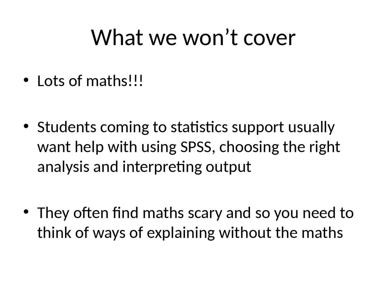
1. Lots of maths!!!Students coming to statistics support usually want help with using SPSS, choosing the right analysis and interpreting outputThey often find maths scary and so you need to think of ways of explaining without the mathsWhat we won’t cover

2. DATA: the answers to questions or measurements from the experimentVARIABLE = measurement which varies between subjects e.g. height or genderData and variablesOne row per subjectOne variable per column

3. Data types

4. Data types

5. Taking a sample from a populationPopulations and sampleswww.statstutor.ac.ukSample data ‘represents’ the whole population

6. Population mean Population SDwww.statstutor.ac.ukPoint estimationsample meanSample SD Sample data is used to estimate parameters of a populationStatistics are calculated using sample data.Parameters are the characteristics of population data estimates  

7. “outliers”minority cases, so different from the majority that they merit separate considerationare they errors?are they indicative of a different pattern?think about possible outliers with care, but beware of mechanical treatments…significance of outliers depends on your research interests

8.

9. summaries of distributionsgraphic vs. numericgraphic may be better for visualizationnumeric are better for statistical/inferential purposes

10. general characteristicskurtosis‘leptokurtic’ ’platykurtic’[“peakedness”]

11. right(positive) skewleft(negative) skewskew (skewness)

12.

13. Descriptive StatisticsClass A--IQs of 13 Students 102 115 128 109 131 89 98 106 140 119 93 97110Class B--IQs of 13 Students127 162131 10396 11180 109 93 87120 105109An Illustration:Which Group is Smarter?Each individual may be different. If you try to understand a group by remembering the qualities of each member, you become overwhelmed and fail to understand the group.

14. Descriptive StatisticsWhich group is smarter now?Class A--Average IQ Class B--Average IQ 110.54 110.23They’re roughly the same!With a summary descriptive statistic, it is much easier to answer our question.

15. Descriptive Statistics Types of descriptive statistics:Organize DataTablesGraphsSummarize DataCentral TendencyVariation

16. Descriptive Statistics Types of descriptive statistics:Organize DataTablesFrequency DistributionsGraphsBar Chart or HistogramFrequency Polygon

17. Frequency DistributionFrequency Distribution of IQ for Two Classes IQ Frequency 82.00 1 87.00 1 89.00 1 93.00 2 96.00 1 97.00 1 98.00 1 102.00 1 103.00 1 105.00 1 106.00 1 107.00 1 109.00 1 111.00 1 115.00 1 119.00 1 120.00 1 127.00 1 128.00 1 131.00 2 140.00 1 162.00 1 Total 24

18. Descriptive Statistics Summarizing Data:Central Tendency (or Groups’ “Middle Values”)MeanMedianModeVariation (or Summary of Differences Within Groups) RangeInterquartile RangeVarianceStandard Deviation

19. Mean Most commonly called the “average.”Add up the values for each case and divide by the total number of cases.Y-bar = (Y1 + Y2 + . . . + Yn) nY-bar = Σ Yi n

20. Mean What’s up with all those symbols, man?Y-bar = (Y1 + Y2 + . . . + Yn) nY-bar = Σ Yi nSome Symbolic Conventions in this Class:Y = your variable (could be X or Q or  or even “Glitter”)“-bar” or line over symbol of your variable = mean of that variableY1 = first case’s value on variable Y“. . .” = ellipsis = continue sequentially Yn = last case’s value on variable Yn = number of cases in your sampleΣ = Greek letter “sigma” = sum or add up what follows i = a typical case or each case in the sample (1 through n)

21. MeanClass A--IQs of 13 Students 102 115 128 109 131 89 98 106 140 119 93 97110Class B--IQs of 13 Students127 162131 10396 11180 109 93 87120 105109Σ Yi = 1437 Σ Yi = 1433Y-barA = Σ Yi = 1437 = 110.54 Y-barB = Σ Yi = 1433 = 110.23 n 13 n 13

22. MeanMeans can be badly affected by outliers (data points with extreme values unlike the rest) Outliers can make the mean a bad measure of central tendency or common experienceAll of UsBill GatesMean OutlierIncome in the U.S.

23. Median The middle value when a variable’s values are ranked in order; the point that divides a distribution into two equal halves.When data are listed in order, the median is the point at which 50% of the cases are above and 50% below it.The 50th percentile.

24. MedianMedian = 109 (six cases above, six below)Class A--IQs of 13 Students 89 93 97 98 102 106 109 110 115 119 128 131 140

25. MedianMedian = 109.5109 + 110 = 219/2 = 109.5(six cases above, six below)If the first student were to drop out of Class A, there would be a new median: 89 93 97 98 102 106 109 110 115 119 128 131 140

26. Median The median is unaffected by outliers, making it a better measure of central tendency, better describing the “typical person” than the mean when data are skewed.All of UsBill Gates outlier

27. MedianIf the recorded values for a variable form a symmetric distribution, the median and mean are identical.In skewed data, the mean lies further toward the skew than the median.MeanMedianMeanMedianSymmetricSkewed

28. Median The middle score or measurement in a set of ranked scores or measurements; the point that divides a distribution into two equal halves.Data are listed in order—the median is the point at which 50% of the cases are above and 50% below.The 50th percentile.

29. Mode The most common data point is called the mode.The combined IQ scores for Classes A & B:80 87 89 93 93 96 97 98 102 103 105 106 109 109 109 110 111 115 119 120127 128 131 131 140 162BTW, It is possible to have more than one mode!A la mode!!

30. ModeIt may mot be at the center of a distribution.Data distribution on the right is “bimodal” (even statistics can be open-minded)

31. ModeIt may give you the most likely experience rather than the “typical” or “central” experience.In symmetric distributions, the mean, median, and mode are the same.In skewed data, the mean and median lie further toward the skew than the mode.MedianMeanMedianMeanModeModeSymmetricSkewed

32. Descriptive Statistics Summarizing Data:Central Tendency (or Groups’ “Middle Values”)MeanMedianModeVariation (or Summary of Differences Within Groups) RangeInterquartile RangeVarianceStandard Deviation

33. RangeThe spread, or the distance, between the lowest and highest values of a variable.To get the range for a variable, you subtract its lowest value from its highest value.Class A--IQs of 13 Students 102 115 128 109 131 89 98 106 140 119 93 97110Class A Range = 140 - 89 = 51Class B--IQs of 13 Students127 162131 10396 11180 109 93 87120 105109Class B Range = 162 - 80 = 82

34. Interquartile RangeA quartile is the value that marks one of the divisions that breaks a series of values into four equal parts.The median is a quartile and divides the cases in half.25th percentile is a quartile that divides the first ¼ of cases from the latter ¾.75th percentile is a quartile that divides the first ¾ of cases from the latter ¼.The interquartile range is the distance or range between the 25th percentile and the 75th percentile. Below, what is the interquartile range?0 250 500 750 100025% of cases25%25%25% of cases

35. VarianceA measure of the spread of the recorded values on a variable. A measure of dispersion.The larger the variance, the further the individual cases are from the mean.The smaller the variance, the closer the individual scores are to the mean.MeanMean

36. VarianceVariance is a number that at first seems complex to calculate.Calculating variance starts with a “deviation.” A deviation is the distance away from the mean of a case’s score.Yi – Y-bar

37. VarianceThe deviation of 102 from 110.54 is? Deviation of 115?Class A--IQs of 13 Students 102 115 128 109 131 89 98 106 140 119 93 97110 Y-barA = 110.54

38. VarianceThe deviation of 102 from 110.54 is? Deviation of 115? 102 - 110.54 = -8.54 115 - 110.54 = 4.46Class A--IQs of 13 Students 102 115 128 109 131 89 98 106 140 119 93 97110 Y-barA = 110.54

39. VarianceWe want to add these to get total deviations, but if we were to do that, we would get zero every time. Why?We need a way to eliminate negative signs.Squaring the deviations will eliminate negative signs...A Deviation Squared: (Yi – Y-bar)2Back to the IQ example, A deviation squared for 102 is: of 115:(102 - 110.54)2 = (-8.54)2 = 72.93 (115 - 110.54)2 = (4.46)2 = 19.89

40. VarianceIf you were to add all the squared deviations together, you’d get what we call the “Sum of Squares.”Sum of Squares (SS) = Σ (Yi – Y-bar)2SS = (Y1 – Y-bar)2 + (Y2 – Y-bar)2 + . . . + (Yn – Y-bar)2

41. VarianceClass A, sum of squares:(102 – 110.54)2 + (115 – 110.54)2 +(126 – 110.54)2 + (109 – 110.54)2 +(131 – 110.54)2 + (89 – 110.54)2 +(98 – 110.54)2 + (106 – 110.54)2 +(140 – 110.54)2 + (119 – 110.54)2 +(93 – 110.54)2 + (97 – 110.54)2 +(110 – 110.54) = SS = 2825.39Class A--IQs of 13 Students 102 115 128 109 131 89 98 106 140 119 93 97110Y-bar = 110.54

42. VarianceThe last step…The approximate average sum of squares is the variance.SS/N = Variance for a population.SS/n-1 = Variance for a sample.Variance = Σ(Yi – Y-bar)2 / n – 1

43. VarianceFor Class A, Variance = 2825.39 / n - 1 = 2825.39 / 12 = 235.45How helpful is that???

44. Standard DeviationTo convert variance into something of meaning, let’s create standard deviation.The square root of the variance reveals the average deviation of the observations from the mean.s.d. = Σ(Yi – Y-bar)2 n - 1

45. Standard DeviationFor Class A, the standard deviation is: 235.45 = 15.34The average of persons’ deviation from the mean IQ of 110.54 is 15.34 IQ points.Review:1. Deviation2. Deviation squared3. Sum of squares4. Variance5. Standard deviation

46. Standard DeviationLarger s.d. = greater amounts of variation around the mean. For example: 19 25 31 13 25 37 Y = 25 Y = 25 s.d. = 3 s.d. = 6s.d. = 0 only when all values are the same (only when you have a constant and not a “variable”)If you were to “rescale” a variable, the s.d. would change by the same magnitude—if we changed units above so the mean equaled 25, the s.d. on the left would be 3, and on the right, 6 Like the mean, the s.d. will be inflated by an outlier case value.

47. Standard DeviationNote about computational formulas:A book provides a useful short-cut formula for computing the variance and standard deviation. This is intended to make hand calculations as quick as possible. They obscure the conceptual understanding of our statistics.SPSS and the computer are “computational formulas” now.

48. Practical Application for Understanding Variance and Standard DeviationEven though we live in a world where we pay real MONEY IN RUPEES for goods and services (not percentages of income), most INDIAN employers issue raises based on percent of salary. Why do supervisors think the most fair raise is a percentage raise?Answer: 1) Because higher paid persons win the most money. 2) The easiest thing to do is raise everyone’s salary by a fixed percent.If your budget went up by 5%, salaries can go up by 5%.The problem is that the flat percent raise gives unequal increased rewards. . .

49. Practical Application for Understanding Variance and Standard DeviationTANDROOST Toilet Cleaning Services Salary Pool: Rs. 200,000Incomes:President: Rs. 100K; Manager: 50K; Secretary: 40K; and Toilet Cleaner: 10KMean: Rs. 50KRange: Rs. 90KVariance: Rs. 1,050,000,000 These can be considered “measures of inequality”Standard Deviation: Rs. 32.4KNow, let’s apply a 5% raise.

50. Practical Application for Understanding Variance and Standard DeviationAfter a 5% raise, the pool of money increases by Rs.10K to Rs.210,000Incomes:President: Rs.105K; Manager: 52.5K; Secretary: 42K; and Toilet Cleaner: 10.5KMean: Rs.52.5K – went up by 5%Range: Rs.94.5K – went up by 5%Variance: Rs.1,157,625,000 Measures of InequalityStandard Deviation: Rs.34K –went up by 5%The flat percentage raise increased inequality. The top earner got 50% of the new money. The bottom earner got 5% of the new money. Measures of inequality went up by 5%.Last year’s statistics:TANDROOST Toilet Cleaning Services annual payroll of Rs.200KIncomes:Rs.100K, 50K, 40K, and 10KMean: Rs.50KRange: Rs.90K; Variance: Rs.1,050,000,000; Standard Deviation: Rs.32.4K

51. Descriptive Statistics Summarizing Data:Central Tendency (or Groups’ “Middle Values”)MeanMedianModeVariation (or Summary of Differences Within Groups) RangeInterquartile RangeVarianceStandard Deviation…Wait! There’s more

52. Box-PlotsA way to graphically portray almost all the descriptive statistics at once is the box-plot.A box-plot shows: Upper and lower quartiles Mean Median Range Outliers

53. Box-Plots123.596.5106.582162M=110.5IQR = 27; There is no outlier.

54. The Data2 Regions – Monthly Sales

55. The CalculationsCalculate Min, Max, Median, Quartile 1 and Quartile 3

56. Calculate Box Heights

57. SAMPLINGSampling denotes the selection of a part of the aggregate statistical material with a view to obtaining information about the whole. This aggregate or totality of statistical information on a particular character of all the members covered by an investigation, is called population.

58. Types of samplingSimple random, Stratified, Systematic, Cluster, and Multistage.Simple randomIt is the simplest of all sampling techniques where all units in a population has equal chance of being included in the sample.There are two methods:1. With replacement ; 2. Without replacement In ‘with replacement’ method, the probability of selection of any particular number of the population at any drawing remains a constant 1/N; because before any draw the population contains all the N members.Interestingly, this result is also true in without replacement method, although the population size varies at each stage of selection. Thus the probability of obtaining the population member Xk (suppose) at the ith draw is a constant 1/N in both the cases i.e., P(Xi=Xk)=1/N for i=1,2,…..n and K=1,2,……N.

59.

60. Random number series - 198 65 33 98 9389 67 42 62 787 60 72 79 4875 14 22 78 2651 11 78 11 8269 70 90 50 7641 1 8 72 1510 28 33 47 2135 61 80 13 118 59 81 91 3079 41 79 35 15100 98 58 8 7598 51 27 34 6185 46 41 79 6931 81 28 33 9195 46 44 87 1529 46 85 82 2617 32 17 57 9499 12 93 69 1557 28 30 47 47

61. Random number series – 2297 42 299 26 198117 169 284 112 81273 15 198 58 11366 33 122 138 60214 281 279 44 114293 156 237 39 142256 13 197 98 149140 214 163 15 91108 165 203 274 15080 241 47 79 269

62. Stratified sampling is generally used when the population is heterogeneous, but can be subdivided into strata within each of which the heterogeneity is not so prominent. Some prior knowledge is necessary for subdivision, termed as stratification. If a proper stratification can be made such that the strata differ from one another as much as possible, but there is much homogeneity within each of them, then a stratified sample will yield better estimates than a random sample of the same size. This is because in stratified sampling different sections of population are suitably represented through the sub samples, which in random sampling some of these sections may be over or under represented or may even be omitted.

63. The principle purpose of stratification are –To increase the overall estimates, To ensure that all sections of populations are adequately representedTo avoid heterogeneity of the population.

64. Managers36Drivers54Administrative Staff90Production Staff180Solve this problem??A company has a total of 360 employees in four different categories:How many from each category should be included in a stratified random sample of size 20 ?Managers1/18 × 36  =  2Drivers1/18 × 54  =  3Administrative Staff1/18 × 90  =  5Production Staff1/18 × 180  =  10TOTAL  =  20To create a sample of size 20 we need 20/360 or 1/18 of the workforce. So we take this fraction of the number of employees in each category.

65. Systematic sampling: Systematic sampling involves the selection of sample units at equal intervals, after all the units in the population have been arranged in some order. If the population size is finite, the units may be serially numbered and arranged. From the first K of these, a single unit is chosen at random. This unit and every k-th unit thereafter constitutes a Systematic sample. In order to obtain a systematic sample of 500 villages out of 40,000 in Assam, i.e., one out of 80 on an average , all the villages have to be numbered serially. From the first 80 of these a village is selected at random, suppose with the serial number 27. Then the villages with serial numbers 27, 107, 187, 267, 347,…. Constitute the systematic sample. If the characteristics under study is independent of the order of arrangement of the units, then a systematic sample is practically equivalent to a random sample. The actual selection of the sample is easier and quicker. Systematic sampling is suitable when the units are described on serial numbered cards, e.g., workers listed on cards. Then the sample can be drawn easily by looking at the serial numbers. The sample may be biased if there are periodic features associated with the sampling interval.

66. Multi-stage Sampling: Multi-stage Sampling refers to a sampling procedure which is carried out in several stages. The population is divided into large groups , called first stage units. These 1st stage units are again divided into smaller units, called 2nd stage units- the 2nd stage units into 3rd stage units, and so on, until we reach the ultimate units. e.g., in order to introduce a scheme on an experimental basis in the villages, we may have to select a few villages from the whole of the state. If we apply 3 stage sampling, sub-divisions may be used as 1st stage units.

67. Cluster sampling: It involves grouping the population and then selecting the groups or clusters rather than individual elements for inclusion in the sample. Suppose some deptt. Store wishes to sample its credit holders. It has issued its cards to 15000 customers. The sample size is to be kept say 450. For cluster sampling this list of 15000 card holders could be formed into 100 clusters of 150 card holders each. Three clusters might then be selected randomly. The sample size must be larger than simple random sampling to ensure same level of accuracy, because possibilities of both sampling or non-sampling error is more. The clustering approach can make the sampling procedure relatively easier and increase efficiency of field works, specially in the case of personal interviews.

68. Exam marks for 60 students (marked out of 65)mean = 30.3 sd = 14.46How can exam score data be summarised?

69. Mean =Standard deviation (s) is a measure of how much the individuals differ from the meanLarge SD = very spread out dataSmall SD = there is little variation from the meanFor exam scores, mean = 30.5, SD = 14.46Summary statistics

70. IQ is normally distributedAbove averageAverageMean = 100, SD = 15.3

71. 95% of values 95% 1.96 x SD’s from the mean70130100P(score > 130) = 0.02595% of people have an IQ between 70 and 130

72. Charts can be used to informally assess whether data is:Assessing NormalityNormallydistributedOr….SkewedThe mean and median are very different for skewed data.

73. Source: Households Below Average Income: An analysis of the income distribution1994/95 – 2011/12, Department for Work and Pensionswww.statstutor.ac.ukSometimes the median makes more sense! 2/3rd people50% people

74. Choosing summary statisticsWhich average and measure of spread?ScaleNormally distributedMean (Standard deviation)Skewed dataMedian (Interquartile range)CategoricalOrdinal:Median (Interquartile range)Nominal:Mode (None)

75. Hypothesis Testing

76. An objective method of making decisions or inferences from sample data (evidence)Sample data used to choose between two choices i.e. hypotheses or statements about a populationWe typically do this by comparing what we have observed to what we expected if one of the statements (Null Hypothesis) was trueHypothesis testing

77. www.statstutor.ac.ukHypothesis testing FrameworkWhat the text books might say!Always two hypotheses: HA: Research (Alternative) HypothesisWhat we aim to gather evidence ofTypically that there is a difference/effect/relationship etc. H0: Null HypothesisWhat we assume is true to begin withTypically that there is no difference/effect/relationship etc.

78. How could you help a student understand what hypothesis testing is and why they need to use it?Discussion

79. Members of a jury have to decide whether a person is guilty or innocent based on evidence Null: The person is innocentAlternative: The person is not innocent (i.e. guilty)The null can only be rejected if there is enough evidence to doubt iti.e. the jury can only convict if there is beyond reasonable doubt for the null of innocenceThey do not know whether the person is really guilty or innocent so they may make a mistakeCould try explaining things in the context of “The Court Case”?

80. Types of ErrorsStudy reports NO difference(Do not reject H0)Study reports IS a difference(Reject H0)H0 is trueDifference Does NOT exist in populationHA is trueDifference DOES exist in populationControlled via sample size (=1-Power of test)Typically restrict to a 5% Risk= level of significanceProb of this = Power of testType I ErrorXType II ErrorX

81. Steps to undertaking a Hypothesis testSet null and alternative hypothesis Make a decision and interpret your conclusionsDefine study questionCalculate a test statisticCalculate a p-valueChoose a suitable test

82. What does it mean for two categorical variables to be related?Remember that Chi-Square is used to test for a relationship between 2 Categorical variables. Ho: There is no relationship between the variables. Ha: There is a relationship between the variables. If two categorical variables are related, it means the chance that an individual falls into a particular category for one variable depends upon the particular category they fall into for the other variable.Let’s say that we wanted to determine if there is a relationship between religion (Christian, Jew, Muslim, Other) and smoking. When we test if there is a relationship between these two variables, we are trying to determine if being part of a particular religion makes an individual more likely to be a smoker. If that is the case, then we can say that Religion and Smoking are related or associated.

83. The chi-squared test is used when we want to see if two categorical variables are relatedThe test statistic for the Chi-squared test uses the sum of the squared differences between each pair of observed (O) and expected values (E)Chi-squared test statistic

84. TABLE A

85. Chi-Square test for 2-way tablesSuppose we are studying two categorical variables in a population, where the first variable has r levels (i.e. possible outcomes) and the second one has s levels.We can summarize a sample from this population using a table with r rows and c columns.A two-way table, also called contingency table, displays the counts of how many individuals fall into each possible combination of categories of two categorical variables. So, each cell of the table (total number of cells is r xc) represents a combination of categories of the two variables.The following table presents the data on race and smoking. The two variables of interest, race and smoking, have r = 4 and c = 2, resulting in 4x2=8 combinations of categories.RaceNSmokeSmokeCaucasian62075Black24041Hispanic13029Other19038

86. Chi-Square test for 2-way tablesBy considering the number if observation falling into each category, we will see how to test the hypotheses of the form: H0: The two variables are not associated. Ha: The two variables are associated.Two different experimental situations will lead to contingency tables If we have two populations under study, both of which have a particular trait with respect to a categorical variable. In this case the null hypothesis is a statement of homogeneity among the two populations. If we have one population under study, and we are interested to check the relationship between two categorical variables. In this case the null hypothesis is a statement of independence between the two variables. For sufficiently large samples, the same test is appropriate for both of these situations. This test is called chi-square test, and in the following we will go over the steps in for testing the relationship between two variables.

87. Some Notation!For i taking values from 1 to r (number of rows) and j taking values from 1 to c (number of columns), denote: Ri = total count of observations in the i-th row. Cj = total count of observations in the j-th column.Oij = observed count for the cell in the i-th row and the j-th column. Eij = expected count for the cell in the i-th row and the j-th column if the two variables were independent, i.e if H0 was true. These counts are calculated as

88. ExampleE11=(695x1180)/1363 E12=(695x183)/1363E21=(281x1180)/1363 E22=(281x183)/1363E31=(159x1180)/1363 E32=(159x183)/1363E41=(228x1180)/1363 E42=(228x183)/1363RaceNSmokeSmokeTotalCaucasianO11 = 620O12 = 75R1 = 695BlackO21 = 240O22 = 41R2 = 281HispanicO31 = 130O32 = 29R3 = 159OtherO41 = 190O42 = 38R4 = 228TotalC1 = 1180C2 = 183n=1363

89. Chi-Square Analysis DetailsThe 5 Steps in a Chi-Square Test:Step 1: Write the null and alternative hypothesis. H0: There is no relationship between the variables. Ha: There is a relationship between the variables. Step 2: Compute expected values Step 3: Calculate Test Statistic and p-value.The test statistic measure the difference between the observed counts and the expected counts assuming independence.This is called chi-square statistic because if the null hypothesis is true, then it has a chi-square distribution with (r-1)x(c-1) degrees of freedom.

90. Step 3 Cont. Find the p-value.If the χ2- statistic is large, it implies that the observed counts are not close to the counts we would expect to see if the two variables were independent. Thus, ''large'' χ2 gives evidence against the null hypothesis, and supports the alternative.The p-value of the chi-square test is the probability that the χ2- statistic, is as large or larger than the value we obtained if H0 is true. Thus, the p-value for Chi-Square test is ALWAYS the area to the right of the test statistic under the curve, i.e. p-value = P(X> χ2), where X has a chi-square distribution with (r-1)x(c-1) df curve.To get this probability we need to use a chi-square distribution with (r-1)x(c-1) df (Table A). Chi-Square Analysis Details

91. Step 4: Decide whether or not the result is statistically significant.The results are statistically significant if the p-value is less than alpha, where alpha is the significance level (usually α = 0.05).Step 5: Report the conclusion in the context of the situation.The p-value is ______ which is < a, this result is statistically significant. Reject the H0 Conclude that (the two variables) are related.The p-value is ______ which is > a, this result is NOT statistically significant. We cannot reject the H0 Cannot conclude that (the two variables) are related.Chi-Square Analysis Details

92. Detailed ExampleDerek wants to know if the geographical area that a student grew up in is associated with whether or not that the student drinks alcohol. Below are the results he obtained from a random sample of PSU students NoYesTotalBig City 216586Rural 11130141Small Town 18198216Suburban 37345382Total87738825

93. Detailed Example1. Ho: There is no relationship between the geographical area that a student grew up and whether or not that the student drinks alcohol. Ha: There is relationship between the geographical area that a student grew up and whether or not that the student drinks alcohol. 2. To check the conditions we need to calculate the expected counts for each cell. E11 = (R1xC1)/n = (86x87)/825 = 9.07,E12 = (R1xC2)/n = (86x738)/825 = 76.93, …E32 = (R3xC2)/n = ___________________, …

94. Detailed Example3. Chi- Square statistic and P-value: χ2 = sum {(Observed – Expected)2/Expected} = (21-9.07)2/9.07+ (65-76.93)2/76.93 + (11-14.87)2/14.87+ (130-126.13)2/126.13 + (18-22.78)2/22.78+ (198-193.22)2/193.22 + (37-40.28)2/40.28+ (345-341.72)2/341.72 = 20.091 df = (4-1)x(2-1) =3 p-value= P(X> 20.091) < P(Xc> 16.17) = 0.001 (see Table A)4. Since the p-value< 0.05, the test is significant, and we can reject the null.5. We can conclude that there is a relationship between the geographical area that a student grew up and whether or not that the student drinks alcohol.

95. The ship Titanic sank in 1912 with the loss of most of its passengers809 of the 1,309 passengers and crew died= 61.8%Research question: Did class (of travel) affect survival?Example: Titanic

96. Null: There is NO association between class and survivalAlternative: There IS an association between class and survivalChi squared Test?3 x 2 contingency table

97. Same proportion of people would have died in each class!Overall, 809 people died out of 1309 = 61.8%What would be expected if the null is true?

98. Same proportion of people would have died in each class!Overall, 809 people died out of 1309 = 61.8%What would be expected if the null is true?

99. Chi-Squared Test Actually Compares Observed and Expected FrequenciesExpected number dying in each class = 0.618 * no. in class

100. Analyse  Descriptive Statistics  CrosstabsClick on ‘Statistics’ button & select Chi-squaredwww.statstutor.ac.ukUsing SPSS p- valuep < 0.001Test Statistic = 127.859Note: Double clicking on the output will display the p-value to more decimal places

101. We can use statistical software to undertake a hypothesis test e.g. SPSSOne part of the output is the p-value (P)If P < 0.05 reject H0 => Evidence of HA being true (i.e. IS association)If P > 0.05 do not reject H0 (i.e. NO association)Hypothesis Testing: Decision Rule

102. Comparing means

103. T-testsPaired or Independent (Unpaired) Data?T-tests are used to compare two population meansPaired data: same individuals studied at two different times or under two conditions PAIRED T-TESTIndependent: data collected from two separate groups INDEPENDENT SAMPLES T-TEST

104. Paired or unpaired?If the same people have reported their hours for 1988 and 2014 have PAIRED measurements of the same variable (hours)Paired Null hypothesis: The mean of the paired differences = 0 If different people are used in 1988 and 2014 have independent measurementsIndependent Null hypothesis: The mean hours worked in 1988 is equal to the mean for 2014 Comparison of hours worked in 1988 to today

105. Paired DataIndependent GroupsSPSS data entry

106. The t-distribution is similar to the standard normal distribution but has an additional parameter called degrees of freedom (df or v) For a paired t-test, v = number of pairs – 1 For an independent t-test, Used for small samples and when the population standard deviation is not knownSmall sample sizes have heavier tailsWhat is the t-distribution?

107. As the sample size gets big, the t-distribution matches the normal distributionRelationship to normalNormal curve

108. Oneway ANOVAAnalysis of variance is used to test for differences among more than two populations. It can be viewed as an extension of the t-test we used for testing two population means.The specific analysis of variance test that we will study is often referred to as the oneway ANOVA. ANOVA is an acronym for ANalysis Of VAriance. The adjective oneway means that there is a single variable that defines group membership (called a factor). Comparisons of means using more than one variable is possible with other kinds of ANOVA analysis.

109. Why Not Use Multiple T-tests?It might seem logical to use multiple t-tests if we wanted to compare a variable for more than two groups. For example, if we had three groups, we might do three t-tests: group 1 versus group 2, group 1 versus group 3, and group 2 versus group3.However, doing three hypothesis tests to compare groups changes the probability that we are making an error (the alpha error rate). When conducting multiple tests of significance, the chance of making at least one alpha error over the series of tests is greater than the selected alpha level for each individual test. Thus, if we do multiple t-tests on the same variables with an alpha level of 0.05, the chances that we are making a mistake in applying our findings to the population is actually greater than 0.05.

110. Step 1. Assumptions for the TestLevel of measurement of the group variable can be any level of variable that identifies groups.Level of measurement of the test variable is interval.The test variable is normally distributed in the population:skewness and kurtosis between –1.0 and +1.0, ornumber is each group is greater than 10 (central limit theorem)The variances (dispersion) of the groups are equal.

111. Step 2. Hypotheses and alphaThe research hypothesis is that the mean of at least one of the population groups is different from the means of the other groups.The null hypothesis is that the means of all of the population groups are equal.If we don’t have a specific reason for setting the level of significance to a specific probability, we can use the traditional benchmark of 0.05. This means that we are willing to risk making a mistake in our decision to reject the null hypothesis if it only happens once in every 20 decisions, or our decision would be correct 19 out of 20 times.

112. Step 3. Sampling distribution and test statisticIn the ANOVA test, the probability is obtained from the “F” distribution instead of the normal curve distribution.The test statistic is also referred to as the F-ratio or F-test because it follows the f-distribution.

113. Step 4. Computing the Test StatisticConceptually the test statistic is computed in a way similar to the independent samples t-test. Both are computed by dividing the differences in means by the measure of variability among the groups.We identify the probability of the test statistic from the SPSS statistical output.

114. Step 5. Decision and InterpretationIf the probability of the test statistic is less than or equal to the probability of the level of significance (alpha error rate), we reject the null hypothesis and conclude that our data supports the research hypothesis.If the probability of the test statistic is greater than the probability of the level of significance (alpha error rate), we fail to reject the null hypothesis and conclude that our data does not support the research hypothesis.

115. Interpreting Differences in Population MeansIf we fail to reject the null hypothesis, we can state that we found no differences among the means for the population groups for this characteristic. We do not say they are equal.If we reject the null hypothesis, we can conclude that the mean for at least one population group is different from the others. The ANOVA test itself does NOT tell us which group means are different. To determine this, we use a Post Hoc test, such as the Tukey HSD (honestly significant differences), LSD (least significant difference) Post Hoc Test.

116. Post Hoc Test for Difference in MeansJust as we used a post hoc test to identify which cells in a frequency table were responsible for the statistically significant result, we use a post hoc test to identify the differences in pairs of means that produce a statistically significant result in an ANOVA table.We only look at the post hoc test when the probability of the ANOVA statistic causes us to reject the null hypothesis, i.e. the probability of the test statistic is less than the level of significance.The Post Hoc Test may NOT reveal differences among group means even when we reject the null hypothesis in the ANOVA test.

117. Inflation of Type I Error (Alpha)Type I Error: Probability of falsely rejecting null hypothesis when it is true.The only time you need to worry about inflation of Type I error rate is when you look for a lot of effects in your data.The more effects you look for, the more likely it is that you will turn up an effect that doesn't really exist (Type I error!). Doing all possible pair-wise comparisons (t-test) on a one-way ANOVA would increase the overall Type I error rate.

118. ANOVA post hoc Test in SPSS (1)Next step is to examine the distribution of the dependent variable. You can check whether the dependent variable is normally distributed or not in:Analyze > Descriptive Statistics > Descriptives…

119. ANOVA post hoc Test in SPSS (2)After moving [age] into “Variable(s):” box, click “Options…” button to select the distribution statistics.

120. ANOVA post hoc Test in SPSS (3)Select “Kurtosis” and “Skewness” to examine whether [age] is normally distributed or not. Then, click “Continue” and “OK” buttons.

121. ANOVA post hoc Test in SPSS (4)[Age] satisfied the criteria for a normal distribution. The skewness of the distribution (.590) was between -1.0 and +1.0 and the kurtosis of the distribution (-.150) was between -1.0 and +1.0.

122. ANOVA post hoc Test in SPSS (5)You can conduct ANOVA by clicking:Analyze > Compare Means > One-Way ANOVA…

123. ANOVA post hoc Test in SPSS (6)Now, click “Post Hoc…” button to select post hoc test option.

124. ANOVA post hoc Test in SPSS (7)Select “Tukey” in “Equal Variances Assumed” panel.Enter alpha in the “Significance level:” textbox. It is same as the alpha level (.01) in the problem.Then, click “Continue” and “OK” buttons.

125. Data SheetControl MeanS.DevT1MeanS.DevT2MeanS.DevT3MeanS.DevT4MeanS.Dev32321.5034340.4233330.3833320.2535350.3834343332353133333234Arrangement for ANOVATreatmentObservationControl-132Control-234Control-331T2R134T2R234T2R333T3R133T3R233T3R333T4R133T4R232

126. CorrelationCorrelation quantifies the extent to which two quantitative variables, X and Y, “go together.” W hen high values of X are associated with high values of Y, a positive correlation exists. W hen high values of X are associated with low values of Y, a negative correlation exists.Now, we have some data, but How to start?The first step is create a scatter plot of the data.

127. Let us deal with an example!!We use the following data set to illustrate correlational methods. In this cross-sectional data set, each observation represents a district of Assam. The X variable is socioeconomic status measured as the percentage of children in a neighborhood receiving mind day meals at school. The Y variable is the percentage of school children owning bicycle. Twelve districts are considered: XYDistrict(% receiving midday meal)(% owning bicycle)Dhubri5022.1Kokrajahr1135.9Dhemaji257.9Dibrugarh1922.2Morigaon2642.4Kamrup735.8Goalpara813.6Sonitpur5121.4Sivsagar1155.2Darrang233.3Nagaon1932.4Barpeta2538.4

128. A scatter plot of the illustrative data is shown to the right. The plot reveals that high values of X are associated with low values of Y. That is to say, as the number of children receivingY (% of bicycle)X (% of mid day meal)

129. Correlation CoefficientCorrelation coefficients (denoted r) are statistics that quantify the relation between X and Y in unit-free terms. W hen all points of a scatter plot fall directly on a line with an upward incline, r = +1 When all points fall directly on a downward incline, r = -1. Such perfect correlation is seldom encountered. W e still need to measure correlational strength, –defined as the degree to which data point adhere to an imaginary trend line passing through the “scatter cloud.” Strong correlations are associated with scatter clouds that adhere closely to the imaginary trend line. Weak correlations are associated with scatter clouds that adhere marginally to the trend line. The closer r is to +1, the stronger the positive correlation. The closer r is to -1, the stronger the negative correlation. Examples of strong and weak correlations are shown below. Note: Correlational strength can not be quantified visually. It is too subjective and is easily influenced by axis-scaling. The eye is not a good judge of correlational strength. 

130. Oneway ANOVAAnalysis of variance is used to test for differences among more than two populations. It can be viewed as an extension of the t-test we used for testing two population means.The specific analysis of variance test that we will study is often referred to as the oneway ANOVA. ANOVA is an acronym for ANalysis Of VAriance. The adjective oneway means that there is a single variable that defines group membership (called a factor). Comparisons of means using more than one variable is possible with other kinds of ANOVA analysis.

131. Why Not Use Multiple T-testsIt might seem logical to use multiple t-tests if we wanted to compare a variable for more than two groups. For example, if we had three groups, we might do three t-tests: group 1 versus group 2, group 1 versus group 3, and group 2 versus group3.However, doing three hypothesis tests to compare groups changes the probability that we are making an error (the alpha error rate). When conducting multiple tests of significance, the chance of making at least one alpha error over the series of tests is greater than the selected alpha level for each individual test. Thus, if we do multiple t-tests on the same variables with an alpha level of 0.05, the chances that we are making a mistake in applying our findings to the population is actually greater than 0.05.