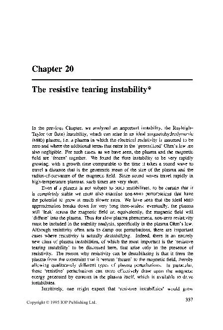
tearing instability* exceedingly slowly, time-scales comparable the ch - PDF document

tearing instability* exceedingly slowly, time-scales comparable the characteristic for resistive magnetic field. little interest, since equilibria are changing such time- scales anyway, the occurrence comparably slowly growing mode practice. However, some resistive instabilities, certainly including the tearing the instability whatever form most efficiently releases the magnetic energy which it Just as the flute instability the plasma energy), the resistive tearing various types the ability energy to lower energy this ‘pent the magnetic trying to to relax to the tearing instability. The one might intuitively the resistive across the magnetic field shorter spatial plasma size and yet energy; because shorter scale-length, can proceed quite quickly. The instabilities, including their surprisingly large growth rates, developed first Phys. Fluids analyze the resistive instability for the simplest current slab’. Specifically, infinite plasma that (or thick current, directed parallel to the surface the slab, Ampere’s law, The functions Figure 20.1. The magnetic plane are illustrated Figure 20.2. the strength different locations the density lines at field is ‘plasma current sheet’ equilibrium. the ‘plasma current sheet’ equilibrium. strong approximately uniform more crowded together. This plasma could possibly be perturbations (although the basic configuration, since the surface element plane (i.e. magnetic field surface element) remain fixed. the inclusion plasma resistivity allow the the left to diffuse into the (or ‘cancelling clearly occur the vicinity is where resistive tearing instability the largest plasma flows resistive tearing instability. to see that this For example, consider the the positive small region energy, s(B:/2)dV, reduced. The actual resistive instability cannot annihilate neat and way: rather wave-like perturbations the entire plasma, the left the magnetic topology near however, the magnetic this type The current-slab configuration illustrated Figure 20.2 additional magnetic present, the plasma can that varies to balance i.e. to the other hand, field is sufficient to balance the functions field will role: as the case the plasma incompressible, satisfying the particular this Chapter, It should these assumptions are made largely analytic simplicity. Resistive instabilities can occur at energetically favored, the equilibrium (or zero) is introduced, that the configuration are considering simply one particular example more general ‘plane Due to magnetic-field vector Such fields said to For sheared the directions can be that the points exactly some selected point, say like the one illustrated Figures 20.1 20.2 (with added). Thus, regard to tearing instabilities, particular example is, Since these plane slab equilibria are and uniform into normal modes the form first-order perturbation quantity. For the equations (20.1) i.e. the k-vector is exactly perpendicular the location with both is clear constant are potential for tearing and we can then direction, subject this being allowed the boundary plane slab are allowed: for extent, the allowed values are determined the boundary which will then limit the surfaces tearing instabilities For the present limit ourselves to the equilibrium only, i.e. simply puts the ‘resonant the location line lies the wave-like perturbation, making the first-order simplify the notation the k-vector. for the remainder the perturbations IDEAL MHD STABILITY CURRENT SLAB our treatment some general properties be obtained from the linearized version Ohm’s law. First, noting that the plasma velocity is zero has only value, denoted Unlike the geometry for considered here the first-order perturbed component arise. provide some combining equation (20.4) the requirement normal mode perturbation quantities as exp(-iwt) are seeking, equation (20.4) written simply drop the from the velocity respectively, since components are zero vanish at any point where example: otherwise, now turn the linearized first-order perturbed equation vector identity linearized the this linearized the second-to-last the right-hand side equation (20.9), to express Just as fact that, (20.9) themselves, have any could obtain for example state. Normally, from the compressible, i.e. incompressible case, determined is substituted into the fluid velocity, i.e. for but this is small quantity that else. Physically, produces whatever modification the almost-uniform magnetic pressure force balance against small flow. Both tearing instability are thus essentially independent plasma pressure. the energy from the inverted density gradient (relative tearing instability can from the sheared magnetic field. however, that this magnetic energy available to the plasma motion only through Just as the two and B,I times the component, equation (20.8). This - - - [B:o: (2-1 - k2ByoB,] Po ax (20.1 0) At this point, our B,o(x) and for the moment, plasma motion this assumption is only approximately valid. validity could the same the perturbation B,I produced strong magnetic relate the force arising from the the perturbed magnetic pressure to either (see, for example, equation (19.22)). Comparing the magnitude this case, is the the case instability, the frequencies the fastest modes that be found here are Hence, again, the compressibility is negligible, approximation write equation (20.11) substitute for equation (20.10) can that this this (PO$) - k2pau,] = & [B:o& ($)I - k2B,oB,. (20.12) For perfect conductivity, equation (20.6) is be used in express the (20.12) also rearranging terms slightly, equation (20.12) Equation (20.14) is homogeneous second-order differential equation for the configuration being proper boundary conditions, eigenmode solutions the equation found. However, certain general properties such waves examining the quadratic equation (20.14) complex conjugate over all The result, after integrating noting that must vanish examining equation (20.15), is evident first that is further evident completely stable (under conductivity), since correspond to pure imaginary value render the equation (20.15) negative-definite, be equal to zero. The stable oscillatory that are described are the the low-frequency limit introduced note that their frequencies are typically is the component wave vector the direction the equilibrium magnetic field. The particular configuration falls into the values assumed equation (20.14) becomes the coefficient derivative can vanish. Since our interest here is stable oscillations, need not explore this is sufficient note that the spectrum possible solutions equation (20.14) contains discrete modes values that are generally subject damping at the location singularity due the ideal introduce resistivity into the plasma Ohm’s law, i.e. Combining this law and linearizing, the magnetic perturbation is have taken the resistivity uniform. Invoking Ampere’s making use Appendix the expansion term on the right-hand side equation (20.3), equation (20.18) becomes have approximated finding that resistivity is important narrow region within which is relatively sharply varying. Equation (20.19) replaces equation the resistive case. The resistive tearing instability Several important conclusions follow treatment corresponds to the For the generally have compared to rates, this the most resistive plasmas. might legitimately perturbation are shorter scale-lengths, that the equation (20.20) are comparable. modes, the resistive equation (20.19) second important conclusion equation (20.19): for the first-order perturbation to vanish at points the particular example 20.2. Physically, relaxing allows the plasma to lower its magnetic energy, corresponding to more the resistive likely to narrow region around the point where particular example. the ‘resistive layer’. Since ‘resonant’ at such that unperturbed magnetic lies parallel to this surface. The the resistive layer then the magnetic connect across the resonance, from the resistive layer, the left and to the particular case Figure 20.1, to remain valid. Since the frequencies appropriately, the growth rates Alfvtn-wave frequencies, the perturbations will be equation (20.14) (or, equivalently, equation (20.12)) but with the inertia terms omitted. describe the perturbations rather than prefer to from equation This equation describes the perturbations to the right from the left from the right), taking the possible forms for are twofold: either Prove the last statement searching for solutions that the first term on the tends to dominate solutions with it safe assume that only these see, however, the case excluded for finite as to multiply equation (20.21) integrate the first term parts, noting localized solution (otherwise there would be which is not case), the first term side vanishes cannot allow this would make limit also, and we would then that the only allowed solutions equation (20.21) are such that approaches some non-zero constant either from the right. Such solutions constraint, i.e. equation (20.6), applied the point Such solutions the resistive replaces equation (20.6) the point where the ‘resistive tearing’ instability. as forming layer’ between the two ideal it. Moreover, obtain some revealing ‘boundary conditions’ integrating various plasma equations Figure 20.3. The box is to have wider than the resistive layer) that is finite the characteristic the perturbation; its extent is arbitrary, since there direction. Integrating the the volume applying Gauss’ theorem, continuous across the boundary, i.e. conditions across at each be constant throughout the Similarly, integrating the surface applying Stokes’s surface integral that any must be ‘surface current’ ‘surface current’, current density narrow layer such that plasma has the capability to carry such the limit zero, the thickness the current approaches zero, surface current arises.) across the note that is continuous across the its gradient Indeed, the quantity quantity Ix~ is seen boundary layer important quantity, which will turn out to tearing modes. the ‘outer-region’ solutions completely determine could imagine integrating equation the left applying the appropriate (or at some intervening boundary, e.g. wall). Indeed, could carry out numerical integration beginning at far to the left, where choose some arbitrary non-zero value for simply measures the amplitude our solution for this region. This solution give some approaching from the left, this value provides alternative measure the amplitude our solution. Thus, choosing some arbitrary value for the amplitude the amplitude the confines the linearized theory), the outer-region solution for completely determined for is the outer-region solution for including the is completely determined intervening conducting wall) the requirement that have the same amplitude, has the solution for the the quantity is completely the outer-region solutions. Indeed, later this Chapter, explicitly for our ‘plasma current configuration, but more detail, to determine how it can provide the localized, concentrated currents needed to produce the sharp that the first-order ‘surface current density’ the perturbed volume current density integrated in across the resistive layer any point is related to the value this point For the particular choice phase in which show that THE RESISTIVE to obtain apply across the resistive layer: it is necessary to resolve the fine-scale structure this layer determine the growth rate resistive tearing mode. the layer, certainly take we may also make use is approximately constant throughout the layer; this constant part will be then becomes side evidently involves resistive layer, since this region, implying that the full equation (20.12) equation (20.12) be simplified noting that the tend to derivatives (i.e. the k-factors) resistive layer. equation (20.12) Substituting for equation (20.27), this becomes have also the result that the tearing instability is the function in the resistive layer. constant, equation (20.29) solved to solution for the Unfortunately, the analytic functions partially numerically. is apparent equation (20.29) away from the resistive layer. Specifically, the left-hand side equation (20.29) negligible. It is also apparent the solution its actual resistive layer form is sketched implicitly assumes that the solution that the homogeneous omitting the no permitted solutions. This established easily, multiplying the integrating from expression that must equal for any solution characteristic width the resistive equation (20.29). Balancing the the left-hand side against the second the right-hand side gives As we expected, the resistive layer becomes thinner as the complete the and find form. For convenient to scaled variables variables, equation (20.29) becomes and, as explicit solution That this is can be direct substitution (20.32), after equations (20.33) we then that equation the asymptotic form for large where the contribution to the integral arises from values that equation (20.33) also asymptotic form, changing the integration variable that the asymptotic for large is obtained analyzing the such detail obtain the conditions to be applied the solutions the left the resistive layer. the previous Section that these outer-region solutions are completely is specified. equations for obtained, for (20.27) across our scaled variables noting that the limits layer width, width, The integral on the right-hand be evaluated numerically, using equation is also possible the integral using both equation (20.33). proceed as as exp(- iX2cos8)(3cos0 - X2cos28)dX 00 (;)I/* g., ~in'/~e(3cos'/~0 - cos'/2e)de (20.3 8) where the final integral evaluated numerically. is equated the previous Section and was the outer-region solutions. Equation expression for the growth Once the quantity calculated from the properties the outer solutions, equation gives the growth rate the resistive tearing reveals some important information about the magnitude the growth interest, it to think the resistivity quantity, i.e. the plasma obeys approximation. The introduction the equilibrium produce diffusion relative to the magnetic field, but only proportional to The introduction non-zero resistivity into stability calculation has, however, modes that grow at faster rate, proportional This argument made more characteristic times. Let characteristic macroscopic e.g. the half-width the current slab characteristic time is the inverse the frequency direction, i.e. almost perpendicular the assumed strong magnetic This shear at the edge the current slab, this second characteristic time describes to non-zero resistivity; since the coefficient’ for this (see, for example, equation this time shows that resistive tearing instabilities grow on time-scales resistive time-scale, the relevant time-scale is close Thus, resistive tearing instabilities resistive tearing instability more slowly instabilities (e.g. the i.e. approaching for finite this discussion, have implicitly order unity, valid, since the macroscopic configuration. this assumption is confirmed, for example, the case current slab THE OUTER MHD REGIONS Until this made use specific form the narrow layer around explicit solution for the form the outer-regions the particular case current slab illustrated Figure 20.1 equations (20.1) solve equation (20.21) for the particular equation (20.2). First consider the region constant. Here, equation (20.2 1) becomes an arbitrary that measures the amplitude the perturbation. equation (20.21) takes the form consider the the a (-)I Bx -k2xB, =O ax ax x but the derivative term can be that equation (20.45) also becomes general solution are arbitrary constants. conditions are obtained from equation the outer region, and they The solutions two regions must latter following from integrating equation For the the two these relations, can easily be obtained the solution One arbitrary must remain, the form the equilibrium to the is exactly the the right the solution be obtained have already the solution is the same the constants calculate the Substituting for equation (20.51), resistive tearing tearing ()- 2ka + 11 exp(-2ka) + 2ka - 1 A’a = (20.55) ‘ In Figure 20.5, plot the (long wavelengths I I describing tearing-mode the condition for the shown that current slab’ equilibrium are wave-like have sufficiently saw at Chapter, the annihilation the cancellation positive and small region energetically favored, it lowers magnetic energy. magnetic perturbation that direction is required to produce the the negative connect to, annihilate, the positive This wave-like perturbation necessarily involves bending field lines, amount that increases as the wavelength decreases. Thus not be the resistive tearing mode sufficiently long the energy released annihilation exceeds that needed this Chapter with both susceptible to resistive instabilities at the boundary conditions. This has an the ‘cylindrical approximately uniform axial weaker azimuthal infinitely long the form ik,z), where can have value. However, the tokamak cylinder is ‘straightened out’ torus be considered have finite length the major (larger) radius Moreover, ‘periodic conditions’ should must take (the choice negative sign being simply for convenience, as integers are allowed). Such perturbation can can ()= m/n. This is the the resonant our ‘slab’ calculation current distribution that peaks decreases to the plasma the function minimum value maximum value rational numbers in’ between have seen that only large wavelengths tend tearing modes, only ‘low-order’ i.e. those for which unstable mode tokamak is that nonlinear evolution this mode tends to strongly flatten the plasma profiles the resonant however, this mode is also dangerous, since can occur whenever particular mode is determined the presence the associated resonant the form current distribution; into our current slab the generalization expect the stable? Is MAGNETIC ISLANDS The resistive the topology the magnetic magnetic configuration current slab instability is illustrated Figure 20.2. The lines are straight strong approximately uniform added to 20.2, lie component reverses After onset the instability, magnetic configuration is deformed, the field lie on are still direction (since there is no the perturbation but which intersect the lines determined the relations the deformed lines project direction onto curved lines the configuration illustrated modified to equilibrium value, complex ones such some particular time the quantity layer around can then where different values constant give The solutions can easily is illustrated 20.6. At relatively large values large values lines are only slightly distorted from the unperturbed configuration Figure 20.2. However, the distortion increases for smaller values smaller values the constant equation (20.58), eventually the lines become 'closed from values constant less for these values the constant equation (20.58) does any real regions shown called 'magnetic When the strong approximately uniform Magnetic islands line configuration The pattem is repeated the individual will not actually close on themselves, but will approximate elliptical cylinders, this case, Figure 20.6 depicts the intersections these surfaces equivalently, the projection lines onto this plane. same surface, its projection onto the plane at traverse the closed curves Figure 20.6 over over again proceeds further The surface line surfaces from the line surfaces is called the 'magnetic separatrix'. The separatrix corresponds to the constant equation (20.58) exactly equal the magnetic island formed course the largest magnetic (see Figure 20.6), the value equation (20.58) for this value the constant the magnetic is proportional the square-root it increases exponentially equation (20.59). practice, nonlinear effects limit the growth resistive tearing instability* the underlying based. Such effects begin to appear as becomes comparable this present can affect the gross current reduce the value the tearing mode. connection between the magnetic islands magnetic separatrix obtained the islands maps presented Indeed, the line equation motion, equation map, where laid down direction. The shear the magnetic the sheared particle and many previous results carry through. The example, scales the square-root some cases, smaller islands, amplitude grows large that secondary islands the primary island or, where several different modes primary island the magnetic When this line can completely across the plasma (i.e. direction for the plasma configuration considered that electron thermal conduction parallel to field will the electron temperature across stochastic region. name ‘tearing mode’ is apparent. The configuration illustrated ‘tears’ at its weakest points, the plane conditions for instability are satisfied (i.e. positive the plasma current slab then have tendency to break into discrete current ‘filaments’. implies that perturbed current density direction is the point in Figure the X-point the island, the point in Figure noted that this is a special property choice of in a cylindrical this for the slab a different method, as follows. Consider magnetic flux ‘trapped’ magnetic island. we may view this field crossing the between the the 0-point; per employing the usual combination Faraday’s law and Ohm’s field is in the the 0-point and the X-point, precludes convection the boundaries the surface under consideration.) The trapped increase as the instability and island-width grow. What does this tell the perturbed current density the island the X-point? resistive tearing the previous Chapter, important instability, the flute) instability, can arise an ideal plasma, i.e.