PDF-The amount of light coming to the eye from an object depends on the amount of light striking

Author : faustina-dinatale | Published Date : 2014-12-16

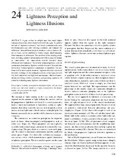
If a visual system only made a single measurement of luminance acting as a pho tometer then there would be no way to distinguish a white surface in dim light from

Presentation Embed Code

<iframe width="560" height="315" src="https://www.docslides.com/embed/24796" frameborder="0" allowfullscreen></iframe>

Download Presentation

Download Presentation The PPT/PDF document "The amount of light coming to the eye fr..." is the property of its rightful owner. Permission is granted to download and print the materials on this website for personal, non-commercial use only, and to display it on your personal computer provided you do not modify the materials and that you retain all copyright notices contained in the materials. By downloading content from our website, you accept the terms of this agreement.

The amount of light coming to the eye from an object depends on the amount of light striking: Transcript

Download Document

Here is the link to download the presentation.
"The amount of light coming to the eye from an object depends on the amount of light striking"The content belongs to its owner. You may download and print it for personal use, without modification, and keep all copyright notices. By downloading, you agree to these terms.