Chapter 13: Effect Sizes and Power

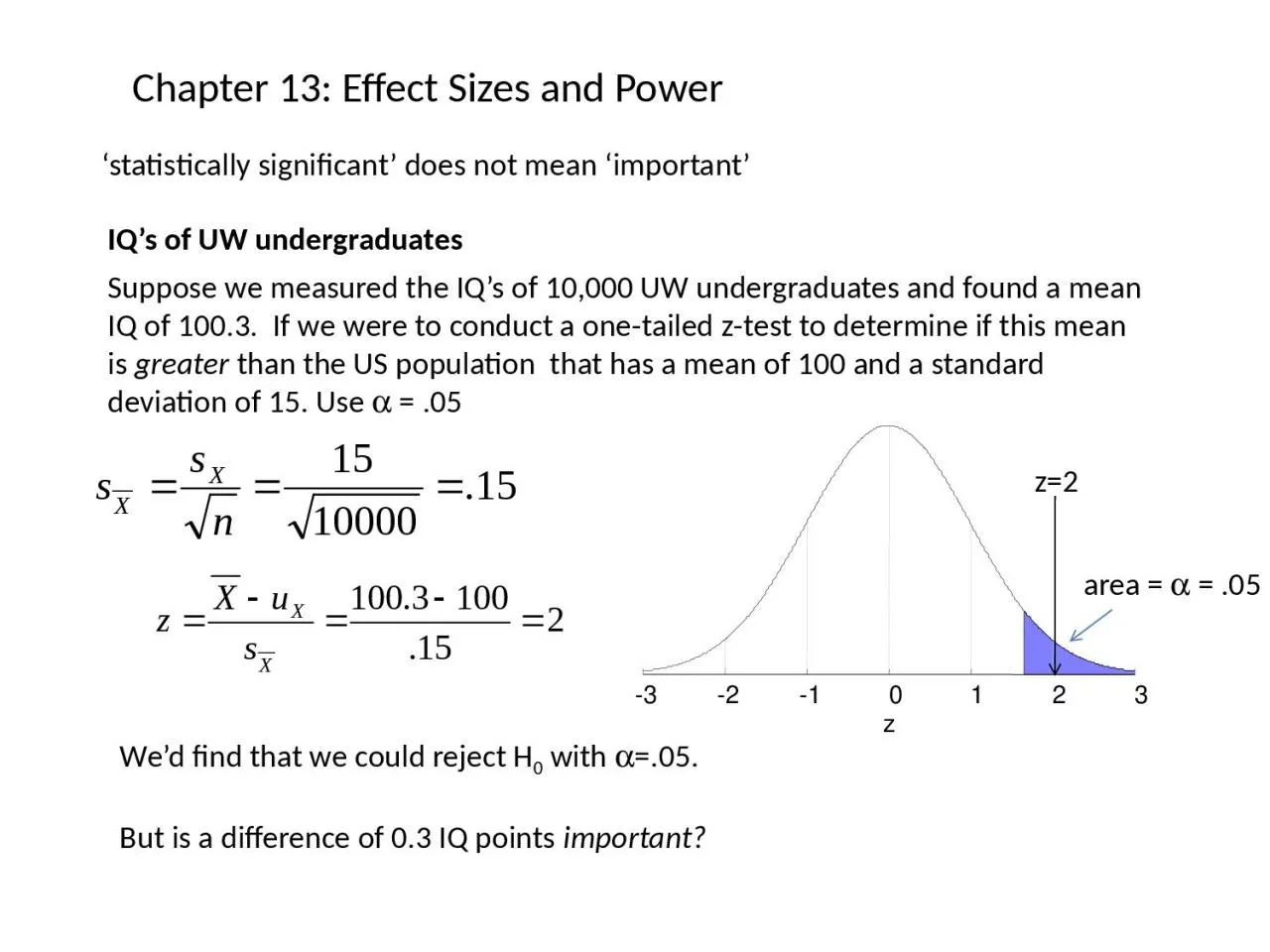
statistically significant does not mean important IQs of UW undergraduates Suppose we measured the IQs of 10000 UW undergraduates and found a mean IQ of 1003 If we were to conduct a onetailed ztest to determine if this mean is

Embed this Presentation

Download Notice

Download Presentation The PPT/PDF document "Chapter 13: Effect Sizes and Power" is the property of its rightful owner. Permission is granted to download and print the materials on this website for personal, non-commercial use only, and to display it on your personal computer provided you do not modify the materials and that you retain all copyright notices contained in the materials. By downloading content from our website, you accept the terms of this agreement.