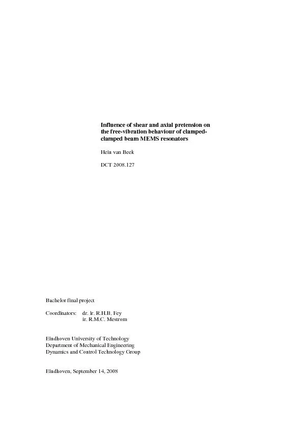
Influence of shear and axial pretension on the free-vibration behaviou - PDF document

Influence of shear and axial pretension on the free-vibration behaviour of clamped-clamped beam MEMS resonators Hein van Beek DCT 2008.127 Bachelor final project Coordinators: dr. ir. R.H.B. Fey ir. R.M.C. Mestrom Eindhoven University of Technology Department of Mechanical Engineering Dynamics and Control Technology Group Eindhoven, September 14, 2008 i Summary Goal A clamped-clamped beam MEMS resonator may be used as a time reference in the near future. For accurate timekeeping, it is important that the frequency at which the micro beam vibrates is very well known. Therefore a model needs to be developed that can accurately predict this natural frequency. In this project is investigated if shear and axial pretension need to be taken in account in such a model. Method In order to investigate the influence of shear and pretension on the mode shapes and the natural frequencies of the clamped-clamped beam MEMS resonator, the project has been divided into four different cases: cases with and without shear and with and without pretension. An Euler beam model is used for the cases without shear and a Timoshenko beam model is used for the cases with shear. Pretension is based on temperature differences. From literature it is known, that shear starts to play a role from a Height/Length ratio of around 1/10. Since the micro beam has this H/L ratio, different H/L ratios are also investigated at all cases to investigate their influence. Different calculation methods, both analytic as FEM based, are used to check for the correctness of the results. Results Regarding the natural frequencies, the influence of shear has been found to be small at low H/L ratios and big at higher H/L ratios, which is according to the expectation. The influence of shear is also increasing at higher eigenmodes. The influence of pretension has been found to be reasonably small at low H/L ratios and very small at higher H/L ratios. The influence of pretension decreases at higher eigenmodes. Regarding the mode shapes, it has been found that the mode shapes are independent of shear and pretension. Numerical problems have been encountered in plotting the mode shapes of the case with shear and with pretension. Conclusions The accuracy requirements in terms of calculating natural frequencies of the model for both shear and pretension are very strict, in the order of ppm. The influence of shear and pretension has been found to be small, but cannot be neglected. Therefore, the model that predicts the frequency of the MEMS resonator should take both shear and pretension into account. The analytic calculation method has been proven to be the best. It is recommended for further research in this topic to solve the numerical problems that have been encountered. ii Table of contents Summary i 1 Introduction 1 2 Clamped-clamped beam MEMS resonator 2 3 Modelling 3 3.1 Model of the MEMS resonator 3 3.2 Modelling approach 3 4 Theoretical background 4 4.1 Euler-Bernoulli 4 4.1.1 Assumptions and differential equation 4 4.1.2 Mode shapes and natural frequencies 5 4.2 Timoshenko 6 4.2.1 Assumptions and differential equations 6 4.2.2 Mode shapes and natural frequencies 7 4.3 Pretension 9 4.3.1 Determining the range of pretensions 9 4.3.2 Effect of pretension on Euler model 10 4.3.3 Effect of pretension on Timoshenko model 11 4.4 Finite Element Methods 13 4.4.1 FEM using Matlab 14 4.4.2 FEM using Marc-Mentat 14 5 Analytical and numerical analysis 16 5.1 Euler without pretension 16 5.1.1 Case 1: Natural frequencies 16 5.1.2 Case 1: Mode shapes 17 5.2 Timoshenko without pretension 18 5.2.1 Case 2: Natural frequencies 18 5.2.2 Case 2: Mode shapes 19 5.3 Euler with pretension 20 5.3.1 Case 3: Natural frequencies 20 5.3.2 Case 3: Mode shapes 22 5.4 Timoshenko with pretension 23 5.4.1 Case 4: Natural frequencies 23 5.4.2 Case 4: Mode shapes 24 5.5 Comparison between the four cases 27 5.5.1 Comparison of the natural frequencies 27 5.5.2 Comparison of the mode shapes 30 6 Conclusions and recommendations 31 Bibliography 32 iii Appendices A Nomenclature 33 A.1 Latin symbols 33 A.2 Greek symbols 34 B Derivation of mode shape coefficients 35 B.1 Mode shape coefficients Timoshenko without pretension 35 B.2 Mode shape coefficients Timoshenko with pretension 36 C Matlab files 38 C.1 Euler without pretension 38 C.2 Euler without pretension FEM 39 C.3 Timoshenko without pretension 40 C.4 Timoshenko without pretension FEM 42 C.5 Euler with compressive pretension 44 C.6 Euler with tensile pretension 45 C.7 Timoshenko with compressive pretension 47 1 1 Introduction A MEMS resonator is a small electro-mechanical device that can be used as a time reference in the near future. MEMS stands for Micro-Electro-Mechanical System. The resonator consists of a clamped-clamped micro beam that vibrates at very high frequencies, along with some sensing and actuation circuitry. To obtain accurate timekeeping, it is important that the frequency at which the beam vibrates is very well known. Therefore, a model is needed that can accurately predict this frequency. Since the resonator is operated in vacuum, the system is very weakly damped. Measurements have also shown this. Therefore, the undamped free vibration is analysed, i.e. the undamped natural frequencies and mode shapes are determined. Of special interest is, whether shear and axial pretension affect the natural frequencies and mode shapes such, that they should be taken in account in the model that is used to predict the frequency of the MEMS resonator. The main goal of this Bachelor Final Project is to find this out. Therefore, the problem has been split up into four cases: with and without shear and with and without pretension. An Euler beam model is used for the cases where shear is neglected, a Timoshenko beam model is used for the cases where shear is taken in account. Pretension is based on temperature differences that may occur in a MEMS resonator during operation. Different calculation methods are used for determining the natural frequencies and mode shapes. Both FEM based methods and (semi-)analytic methods are used. This allows for checking of the correctness of the results. Eventually, this may lead to the conclusion that one method is preferred over the others. In summary, the problem definition for this project is the following: ‘What is the influence of shear and axial pretension on the free-vibration behaviour of clamped-clamped beam MEMS resonators?’ A short outline of this report is as follows. In chapter 2, more information about the specific MEMS resonator under investigation can be found. Chapter 3 deals with the modelling approach that is used in this project. In chapter 4, the theoretical background on the different modelling approaches in this project is discussed. Chapter 5 deals with the analysis of the results of this project. In chapter 6 the conclusions and recommendations can be found. 2 2 Clamped-clamped beam MEMS resonator A MEMS (Micro-Electro-Mechanical System) resonator is a small device that consists of a vibrating micro beam and some actuation and sensing circuitry, see figure 2.1 and 2.2. It is proposed to be used as a timing device in for example a mobile phone or a computer in the near future. The frequency at which the micro beam vibrates will be used as a reference for the time that passes. To enable accurate timekeeping it is important that the frequency at which the beam vibrates is very well known. Even small deviations may lead to unacceptable differences in the time the beam suggest and the real time. This causes the frequency tolerances of the MEMS resonator to be very strict. An overview of the relevant frequency tolerances are given in table 2.1, adopted from [8]. Furthermore, some physical properties of the MEMS resonator are given in table 2.2. Figure 2.1: MEMS resonator system.Figure 2.2: Close-up of the micro beam.Table 2.1: Overview of the frequency tolerances. Property Tolerance static frequency @ 25° C ± 2 ppm frequency change over temperature range (-20, 100) ° C ± 3 ppm Table 2.2: Physical properties of the MEMS resonator. Property Value Material Silicon Length L 44 m Height H 4 m Width B 1.4 m Density 2330 kg/m3 Young’s modulus E 131 GPa Poisson’s ratio 0.28 Thermal expansion coefficient 4.2e-6 K-1 3 3 Modelling3.1Model of the MEMS resonator A MEMS resonator’s most important part is a vibrating micro beam. The MEMS resonator is modelled as a clamped-clamped beam with length L in x-direction, height H in y-direction and width B in z-direction. This can also be seen in figure 3.1. Figure 3.1: Model of a clamped-clamped beam MEMS resonator. 3.2 Modelling approach Several different models are available for calculating mode shapes and natural frequencies of vibrating beams. Two well-known models are the Euler-Bernoulli beam model and the Timoshenko beam model. The biggest difference between these models is that the Euler-Bernoulli model neglects shear and rotary inertia, while the Timoshenko model takes these two in account. From literature, see for instance [1,2], it is known that for a height / length ratio (H/L ratio) of around 1/10 and at higher modes, shear and rotary inertia effects become important and lead to a significant difference in natural frequencies. Since the dimensions of the beam are such that these effects of shear and rotary inertia may play a role, natural frequencies and eigenmodes are calculated both using the Euler-Bernoulli model and the Timoshenko model. This is done for different H/L ratios, with L constant and H variable. A further point of interest is pretension. Pretension can be caused by manufacturing effects or by temperature differences. In this project, pretension is assumed to be caused by temperature differences. From literature, see [5] or [6], it is known that pretension affects the natural frequencies of vibrating beams, but it is not known whether these effects are significant for micro beams. This will also be investigated in this project, in order to find the effects of pretension on the natural frequencies and mode shapes of the micro beam. As a result, the following modelling approach is proposed, in which four different cases will be investigated: 1.without shear and pretension, different H/L ratios 2.with shear and without pretension, different H/L ratios 3.without shear and with pretension, different H/L ratios, different pretensions 4.with shear and with pretension, different H/L ratios, different pretensions The theoretical background on the different beam models will be described in the next chapter. 4 4 Theoretical backgroundIn this chapter the theoretical background used in this project will be discussed. First, two commonly used beam theories, Euler-Bernoulli and Timoshenko, will be explained regarding the used formulas and assumptions. In paragraph 4.3, the influence of pretension for both the Euler-Bernoulli and the Timoshenko case will be described. Finally, it will be described how the mode shapes and natural frequencies for the two cases can be calculated using Finite Element Method (FEM), using both Matlab and Marc-Mentat. 4.1 Euler-Bernoulli In this project, two commonly used theories to describe the static and dynamic behaviour of beams will be compared, namely Euler-Bernoulli beam theory and Timoshenko beam theory. In this report, these theories will be referred to ‘Euler’ and ‘Timoshenko’. 4.1.1Assumptions and differential equation To describe the static and dynamic behaviour of beams, Euler-Bernoulli beam theory uses the following assumptions: 1.The material of the beam is isotropic. 2.The material behaviour is linear elastic. 3.Rotary inertia is negligible. 4.Shear deformation is negligible. Under these assumptions, the following partial differential equation of motion for small deflections of an Euler beam can be written: 4242 0 yyEIA xt ¶¶ += ¶¶, (4.1) stiffness mass inertia where E is the Young’s modulus or modulus of elasticity [Pa], I is the second moment of area [m], y is de deflection of the beam [m], x is the coordinate along the beam length [m], is the density of the beam material [kg m-3], A is the cross section area [m] and t is the time [s]. When the beam vibrates in one of its natural modes, the deflection y becomes (this is called separation of variables): (,)()cos() yxtYxt w = , (4.2) in which Y(x) is the modal displacement [m] and is the circular natural frequency [rad/s]. This way, the differential equation becomes: 4242 0 dYdYEIA dxdt rw -= . (4.3) 5 4.1.2 Mode shapes and natural frequencies To determine the mode shapes and the natural frequencies of the beam, differential equation (4.3) has to be solved. For a clamped-clamped beam, the boundary conditions are as follows: (0)()0 YYL == , (4.4) and (0)() 0 dYdYL dxdx == . (4.5) The equations can be solved easiest by making them dimensionless. Therefore, a dimensionless beam coordinate [-] is defined as: x L x = . (4.6) By solving the differential equation, a characteristic equation for the natural frequency and a general solution for the mode shapes can be obtained (the way to do this is explained in more detail in the Timoshenko section, chapter 4.2 or can also be found in Blevins [4]). For mode i, the general solution for the mode shapes can be shown to be: ()cosh()cos()(sinh()sin()) iiiiii xlxlxslxlx =---, (4.7) in which [-] is the solution of the characteristic or frequency equation, cos()cosh()1 ll = , (4.8) and [-] a constant depending on : cosh()cos() sinh()sin() ii i ii ll s ll . (4.9) Furthermore, the natural frequency f [Hz] can be obtained by: 222ii EI f A Ll r , (4.10) where L is the length of the beam [m]. 6 4.2 Timoshenko The second model that has been used in this project is the Timoshenko model. It differs from the Euler model in the fact that it takes shear and rotary inertia in account. 4.2.1 Assumptions and differential equations The assumptions in Timoshenko beam theory are the following: 1.The material of the beam is isotropic. 2.The material behaviour is linear elastic. 3.Rotary inertia is taken in account. 4.Shear deformation is taken in account. So the Timoshenko model shares the isotropic and linear elastic material behaviour assumptions with the Euler model and differs with respect to the inclusion of shear and rotary inertia. These assumptions lead to a system of two coupled partial differential equations, known as: 22 ()0 EIAGI x xt yykyr¶¶¶ +--= ¶ ¶¶ , (4.11) stiffness shear rotary inertia 2222 ()0 yyAAG x tx rk¶¶¶ --= ¶ ¶¶ , (4.12) mass inertia shear where is the rotation of the beam [rad], G is the shear modulus [Pa] and is the shear coefficient [-], which can be found to be for rectangular cross sections (see [4]): 10(1) 1211 n k n + , (3.13) in which is the Poisson’s ratio [-]. A list of all symbols and their meaning can also be found in appendix A. Above system of differential equations can be decoupled as follows, adopted from reference [1]: 42422442224 (1)0 yyEymRyEImmR GAG xtxtt kk¶¶¶¶ +-++= ¶¶¶¶¶ , (4.14) 42422442224 (1)0 EmREImmR GAG xtxtt yyyykk¶¶¶¶ +-++= ¶¶¶¶¶ , (4.15) where R is the radius of gyration [m], I R A , (4.16) and m = A is the mass per length of the beam [kg/m]. According to reference [1], the last term in (4.14) and (4.15) can be omitted due to its negligible contribution to yield: 7 4244222 (1)0 yyEyEImmR G xtxt ¶¶¶ +-+= ¶¶¶¶ , (4.17) 4244222 (1)0 EImmR G xtxt yyy¶¶¶ +-+= ¶¶¶¶ . (4.18) When the beam vibrates in one of its natural modes, the following equivalent forms for the rotation and the deflection y can be used: (,)()cos() yxtYxt w = , (4.19) (,)()cos() xtxt yw =Y , (4.20) where (x) is the modal rotation. The system of differential equation can be solved easiest in dimensionless form, so the following dimensionless parameters are introduced: 24 2 AL p EI rw, R r L = , 2 2 EI b AGL k . (4.21) This way, the system of uncoupled differential equations becomes, as shown by Abramovitch and Elishakoff in [1]: 42222242 ()0 dYdYprbpYddxx ++-= , (4.22) 42222242 ()0 ddprbpddxxYY ++-Y= . (4.23) 4.2.2 Mode shapes and natural frequencies The uncoupled set of differential equations, (4.22) and (4.23), have the following general solutions for the transversal and rotational mode shape, see [1]: 11213242 ()cosh()sinh()cos()sin() YBpsBpsBpsBps xxxxx =+++, (4.24) 11213242 ()cosh()sinh()cos()sin() CpsCpsCpsCps xxxxx Y=+++, (4.25) where B1-4 and C1-4 are constants [-], depending on the mode of the beam and the boundary conditions. The constants s and s [-] can be obtained from: 22222 2 14 ()22rbsrb p =-+++, (4.26) 22222 2 14 ()22rbsrb p =++++, (4.27) and finally, p can be obtained as the solution of the characteristic equation: 8 2224221212222(3()) 22cosh()cos()sinh()sin()0 pbrpbbrpspspspspbr-++ -+= . (4.28) The constants B1-4 and C1-4 are not independent. Following the steps from reference [1], so by substituting the general solutions, (4.24) and (4.25), into the differential equations, (4.17) and (4.18), and taking in account (4.19) and (4.20), the following relations between B1-4 and C1-4 can be found: 22 12 1 () psb CB Ls, 22 21 1 () psb CB Ls, (4.29) 22 34 2 () psb CB Ls, 22 43 2 () psb CB Ls-+. (4.30) Since there is only interest in the transversal mode shape and not in the rotational mode shape, above relations can be used in (4.24) and (4.25), together with the boundary conditions: (0)(1)0 YY == , (4.31) (0)(1)0 Y=Y= , (4.32) to find expressions for B2-4 as a function of B. Since there are four equations, one would probably expect the ability to eliminate all four constants B1-4 in the general equation for the mode shape. However, this cannot be done, for the simple fact that one equation is already used to determine the characteristic (or frequency) equation. The following expressions can be found for B2-4 as a function of B (a derivation of the expressions can be found in appendix B.1): 22 21 222121 sin()sinh() cos()cosh()sb psps sbBBpsps

, (4.33) 31 BB =- , (4.34) 2212 12 224121 sinh()sin() cos()cosh()sbs psps sbBBpsps

=- . (4.35) The value of B can be chosen arbitrarily, but for proper comparison between different mode shapes, it is useful to choose a certain normalization. The normalization chosen in this project is that the maximum value of the mode shape equals 1, so: max()1 Y = . (4.36) Since p is already known from the characteristic equation, the natural frequencies fcan be easily calculated from the definition of p: 9 22i pEI f A L r . (4.37) Note that p is different for each eigenmode. 4.3 Pretension From literature it is known (see for instance [2], [5] or [6]) that pretension affects the mode shapes and the natural frequencies. It is unknown whether these effects are significant for micro beams like in a MEMS resonator. This will be investigated in this project. 4.3.1 Determining the range of pretensions Pretension in the beam assumed to be caused by temperature differences. When temperature increases or decreases compared to the reference temperature, the beam material wants to expand or shrink. Due to the clamped-clamped boundary condition the material however cannot expand or shrink freely. This results in tensile axial pretension in case of a temperature decrease and compressive axial pretension in case of a temperature increase. In Fenner [7] the following formula for calculating the axial pretension can be found: ()xref ETTET saa =--=-D , (4.38) where is the axial pretension [Pa], is the thermal expansion coefficient [K-1], T is the temperature [K], Tref is the reference temperature [K] and T is the temperature difference [K]. The reference temperature is set to room temperature, so 20° C. The range of temperatures is set between -20° C and 100° C (the temperature range in which the MEMS resonator should work properly, see table 2.1). This results in a range of pretensions as listed in table 4.1. Note that a positive pretension indicates tensile stress and a negative pretension indicates compressive stress. Table 4.1: Pretensions at different temperatures. T (°C) T (°C) (MPa) -20 -40 22 0 -20 11 20 0 0 40 20 -11 60 40 -22 80 60 -33 100 80 -44 10 4.3.2 Effect of pretension on Euler model In both the Euler and Timoshenko case, pretension leads to an extra term in the differential equation(s), namely: 22 22 xx yy NA xx s ¶¶ ±=± ¶¶ , (4.39) where N is the axial force. The plus minus sign represents the difference between tensile (-) and compressive (+) pretension. Thus, the partial differential equation in the Euler case becomes: 422422 0 yyyEIAN xtx ¶¶¶ ++= ¶¶¶ , (4.40) for compressive axial pretension and 422422 0 yyyEIAN xtx ¶¶¶ +-= ¶¶¶ , (4.41) in case of tensile axial pretension. These differential equations lead to a characteristic equation for calculating the natural frequencies and a general solution of the differential equation to calculate the mode shapes. These can be derived using exactly the same procedure as has been done in the Timoshenko case without pretension (section 4.2.2), although it becomes a little more complicated due to the extra term. Here, only the resulting characteristic equation and general solution for the mode shapes will be presented, for the derivation, see [5] for the compressive case and [6] for the tensile case. First, the following variables are defined, which help to represent the characteristic equation and the general solution for the mode shapes in an easier way: 2 2 x NL U EI , (4.42) A L EI r W=, (4.43) 22 MUU =-++W , (4.44) 22 NUU =+++W , (4.45) in which U is the relative axial force [-], is the relative circular natural frequency [-] and M and N are mode shape constants [-]. For compressive axially loaded beams, the characteristic equation is as follows: sinh()sin()cosh()cos()0 UMNMN W--W= . (4.46) The mode shapes for the compressive case can be found to be: 11 sin()sinh() ()sinh()(cosh()cos())sin() (cosh()cos())MNNMM YMMNN NMNN xxxxx - =+--. (4.47) For tensile axially loaded beams, the characteristic equation is as follows: sinh()sin()cosh()cos()0 UNMNM W+-W= . (4.48) The mode shapes for the tensile case can be found to be: sin()sinh() ()sinh()(cosh()cos())sin() (cosh()cos())NMMNNYNNMMMNMM xxxxx - =+--. (4.49) It should be noted that both expressions for the mode shapes are not yet normalized. The normalization used in this project is that the maximum of Y equals one. The buckling load Nx,cr [N] can be expressed as: xcr EI N L . (4.50) The buckling stress x,cr [Pa] can be easily found by dividing the buckling load by the cross-sectional area: xcrxcr EI A AL == (4.51) When the pretension is higher than the buckling stress, the beam will buckle and thus, all formulas presented for eigenmodes and natural frequencies are not valid anymore. In table 4.2 the maximum pretension is compared with the buckling stress for various H/L ratios. It can be concluded that the pretension does not exceed or come close to the buckling stress. Therefore, all presented formulas can be used. Table 4.2: Buckling stress for various H/L ratios. H/L ratio (-) x,cr (GPa) x,max (MPa) x,maxx,cr (%) 1/44 -0.2226 -44 19.8 4/44 -3.562 -44 1.24 10/44 -22.26 -44 0.198 4.3.3 Effect of pretension on Timoshenko model As mentioned in the Euler part about pretension, pretension affects the Timoshenko model by introducing an extra term in the differential equations. Unfortunately, there are only expressions available for Timoshenko beams under compressive axial loads and not for tensile axial loads. Therefore, only compressive axial loads for the Timoshenko model will be considered. The system of coupled differential equations for Timoshenko beams under compressive axial loads is as follows: 12 2222 10 yyxGAGxtyrkk¶¶¶
 -+--= ¶¶, (4.52) 22 0 EIGAIxtyykyr¶¶¶
 +--= ¶¶. (4.53) Following the procedure explained in chapter 4.2 (see also [2]), expressions for the mode shapes and natural frequencies can be obtained. First, some parameters are defined: GA ak = , 2 2 I r AL , 2 2 EI b L a , (4.54) NL N EI a =
 -   , 24 AL EIrw a =
 -   , (4.55) in which is the shear load [N], r is the relative radius of gyration [-], b is the stiffness / shear ratio [-], k is the relative axial load and p is the relative natural frequency [-]. Furthermore, s and s [-] are given by: 2 222222222 11 114 22xNN sprbkprbkp aa





=--+++-+++, (4.56) 2 222222222 11 114 22xNN sprbkprbkp aa





=+-+++-+++. (4.57) The characteristic or frequency equation (for determining p) can be found to be: () 242242121222222114 22cosh()cos()sinh()sin()0 11ppbrbkbbsssspbrbk

--++++ -+=
+-+. (4.58) The general solution for the transversal mode shape, obtained from [2], is as follows: 11213242 ()cosh()sinh()cos()sin() YBpsBpsBpsBps xxxxx =+++, (4.59) in which the following expressions for the mode shape coefficients B2-4 can be found as a function of B (see appendix B.2 for the derivation): 1221 12 sinh()sin() cosh()cos() MsNs BB MsMs =-, (4.60) 31 BB =- , (4.61) 13 124112 (sinh()sin()) (cosh()cos()) MMsNs BB NMsMs , (4.62) where M and N are given by: 222 N spb a +
 =-   , (4.63) 222 x N spb a -
 =-   . (4.64) can be obtained by choosing a normalization. In this project, the maximum of the mode shape is set to one, so: 11 max() B Y . (4.65) The expression for the rotational mode shape is abandoned, since it is not of interest in this project (although it is needed for determining the constants B2-4). Finally, the buckling load for the Timoshenko case is given by: 2, 22 4 4 xcr EI p p a . (4.66) For the most important H/L values the maximum axial pretension is compared to the buckling stress (buckling load divided by area). It can be seen that the maximum pretension does not exceed or come close to the buckling stress. Thus, the presented formulas for calculating the natural frequencies and eigenmodes are valid. Table 4.3: Buckling stress for various H/L ratios. H/L ratio (-) x,cr (GPa) x,max (MPa) x,maxx,cr (%) 1/44 -0.2215 -44 19.9 4/44 -3.292 -44 1.33 10/44 -14.72 -44 0.299 4.4 Finite Element Methods Two different FE approaches are used in this project: one uses a self-written FE-program in Matlab and the other uses the commercial FE software package Marc-Mentat. The self written FE program has the advantage that it is exactly known what is done (in terms of formulas used etc.) to calculate mode shapes and natural frequencies. Unfortunately, it is not capable of determining mode shapes and natural frequencies when pretension is applied. Marc-Mentat has as advantage that it can be used in case of pretension, but as disadvantage that it is a black box: some parameters are put in, Marc-Mentat starts calculating and the end results pop up on the computer screen. It is not exactly known how things are calculated. So if inaccurate or false results are generated, it is unknown what causes them, which makes it difficult to improve or compare results. 14 4.4.1 FEM using Matlab With FEM, a structure (a beam in this case) is divided into a finite number of elements. For each of these elements an element mass matrix M and an element stiffness matrix K can be defined. The element stiffness matrix is different for the Euler and Timoshenko model, while the element mass matrix is the same for Euler and Timoshenko. Expressions for these matrices can be found in [3]. The element mass matrices and element stiffness matrices can be assembled to a system mass matrix M and a system stiffness matrix K. By solving the eigenvalue problem: []0 KMu -= , (4.67) natural frequencies and eigenmodes can be determined, where is the circular natural frequency [rad/s] and u is the eigenmode. If the number of elements chosen is sufficiently high, the exact solutions for mode shapes and natural frequencies will be approximated. Matlab is used for assembling the element stiffness and mass matrices into the system stiffness and mass matrices and for solving the eigenvalue problem. It is not possible to use this FE method when pretension is applied, so it is only used for the Euler and Timoshenko case without pretension. 4.4.2 FEM using Marc-MentatMarc-Mentat is also used as FE package for determining the mode shapes and natural frequencies of the micro beam. For the case without pretension, calculating mode shapes and natural frequencies is straightforward. The graphical user interface can be used to draw a beam, to divide it into enough elements, to assign geometric and material properties and the boundary conditions and, as a last step, to use a dynamic modal load case to determine the mode shapes and the natural frequencies. For the Euler case, the 2-node element 5 is used and for the Timoshenko case, the 3-node element 45 is used (see Marc Mentat manual [9]). However, assigning pretension to the beam in Marc-Mentat is not straightforward, since it is not possible to assign stress to an element or putting forces on the beam which should lead to the right pretensions. The method for introducing pretension in the beam is by prescribing a displacement to one end of the beam. Here, the beam starts with an initial length L, different from the designed length L it should have with the right pretension assigned: 011xE LLL es==++, (4.68) where is the strain. As load case in Marc-Mentat, a displacement is prescribed as a fixed value. The displacement and length L must be chosen such that, after displacement, the beam has length L and the desired pretension. Therefore, the displacement x needs to be: 1xx xLL esD==++. (4.69) 15 The other steps for calculating mode shapes and natural frequencies are the same as for the case without pretension. Note that the load cases for the displacement and the dynamic modal analysis must be arranged such that the modal analysis is done after the displacement has been prescribed to the beam. 16 5 Analytical and numerical analysis In the first four sections of this chapter the results of each of the four cases (Euler / Timoshenko, with / without pretension, see also section 3.2) are presented. The results are based on the theory, presented in the previous chapter. Next, in section 5.5, a comparison is made between the four cases. The Matlab scripts that are used to calculate the natural frequencies and eigenmodes can be found in appendix D. 5.1 Case 1: Euler without pretension The first case is the case without shear and without pretension. For different H/L ratios and for all three different calculation methods the mode shapes and natural frequencies are presented. 5.1.1 Case 1: Natural frequencies The first three natural frequencies for the case without shear and without pretension are given in table 5.1. Three different calculation methods are used to calculate the natural frequencies. First, a semi-analytic method is used. This method uses the analytical equations of chapter 4. The method is called semi-analytic because it uses the analytical equations, but they are solved using a numerical solver of Matlab. In the table however, it is named analytic. The second calculation method used is the Marc-Mentat FE software package. In the table, this method is called Marc-Mentat. The third method used is a self written FE program in Matlab. This method is called FEM Matlab in the table. The method values in table 5.1 are calculated using the analytical method. A comparison between the different calculation methods can be found in tables 5.2-5.4 in paragraph 5.2.1. Table 5.1: First three natural frequencies for Euler case without pretension (analytic). H (µm) L (µm) f (MHz) f (MHz) f (MHz) 1 44 3.98118 10.9743 21.5140 2 44 7.96236 21.9485 43.0279 3 44 11.9435 32.9228 64.5419 4 44 15.9247 43.8971 86.0558 5 44 19.9059 54.8714 107.570 6 44 23.8871 65.8456 129.084 7 44 27.8682 76.8199 150.598 8 44 31.8494 87.7942 172.112 9 44 35.8306 98.7684 193.626 10 44 39.8118 109.743 215.140 From table 5.1 some conclusions can be drawn. Firstly, it can be seen that for higher eigenmodes the frequency increases. For thicker beams (H higher) the natural frequency also increases. The linearity of the Euler case also is remarkable: if H is twice or ten times as large, the natural frequency also becomes twice or ten times as large. The reason for this is that the height of the beam appears linearly in the natural frequency equation (4.10): 222222 2212212 iii EIEBHE HLALBHLlll prprpr ===. (5.1) 17 5.1.2Case 1: Mode shapes In figure 5.1 the mode shapes of H/L = 4/44 can be seen. There is hardly any difference between the mode shapes for various H/L ratios. An example of this can be seen in figure 5.2, where for H/L = 1/44, 4/44 and 10/44 the second mode is plotted. 0 0.2 0.4 0.6 0.8 1 -1 -0.8 -0.6 -0.4 -0.2 0 0.2 0.4 0.6 0.8 1 [-] [-] f1 f2 f3 Figure 5.1: Mode shapes for H/L = 4/44. 0 0.2 0.4 0.6 0.8 1 -1 -0.8 -0.6 -0.4 -0.2 0 0.2 0.4 0.6 0.8 1 [-] [-] H/L = 1/44 H/L = 4/44 H/L = 10/44 Figure 5.2: Second mode: comparison between different H/L ratios. 18 5.2 Case 2: Timoshenko without pretension The second case is the case with shear and without pretension. For different H/L ratios and for all three different calculation methods the mode shapes and natural frequencies are presented. 5.2.1 Case 2: Natural frequencies In tables 5.2-5.4 the natural frequencies for various calculation methods can be seen. The natural frequencies are given for both the Euler (E) as the Timoshenko (T) case, so they can be compared. Table 5.2: Natural frequencies f for various calculation methods. Beam dimensions Analytic Marc-Mentat FEM Matlab H (µm) L (µm) f1,E (MHz) f1,T (MHz) f1,E (MHz) f1,T (MHz) f1,E (MHz) f1,T (MHz) 1 44 3.98118 3.96741 3.981 3.969 3.98118 3.96845 2 44 7.96236 7.35387 7.962 7.869 7.96236 7.86194 3 44 11.9435 11.5864 11.94 11.64 11.9435 11.6122 4 44 15.9247 15.1060 15.92 15.22 15.9247 15.1630 5 44 19.9059 18.3716 19.91 18.58 19.9059 18.4734 6 44 23.8871 21.3596 23.89 21.69 23.8871 21.5185 7 44 27.8682 24.0628 27.87 24.55 27.8682 24.2883 8 44 31.8494 26.4865 31.85 27.15 31.8494 26.7849 9 44 35.8306 28.6451 35.83 29.51 35.8306 29.0194 10 44 39.8118 30.5585 39.81 31.63 39.8118 31.0092 Table 5.3: Natural frequencies f for various calculation methods. Beam dimensions Analytic Marc-Mentat FEM Matlab H (µm) L (µm) f2,E (MHz) f2,T (MHz) f2,E (MHz) f2,T (MHz) f2,E (MHz) f2,T (MHz) 1 44 10.9743 10.8868 10.97 10.90 10.9743 10.8975 2 44 21.9485 21.2726 21.95 21.36 21.9485 21.3523 3 44 32.9228 30.7621 32.92 31.04 32.9228 31.0043 4 44 43.8971 39.1242 43.90 39.73 43.8971 39.6263 5 44 54.8714 46.2905 54.87 47.35 54.8714 47.1309 6 44 65.8456 52.3135 65.85 53.93 65.8456 53.5425 7 44 76.8199 57.3145 76.82 59.54 76.8199 58.9569 8 44 87.7942 61.4411 87.79 64.31 87.7942 63.5031 9 44 98.7684 64.8399 98.77 68.34 98.7684 67.3163 10 44 109.743 67.6430 109.7 71.75 109.743 70.5224 Table 5.4: Natural frequencies f for various calculation methods.Beam dimensions Analytic Marc-Mentat FEM Matlab H (µm) L (µm) f3,E (MHz) f3,T (MHz) f3,E (MHz) f3,T (MHz) f3,E (MHz) f3,T (MHz) 1 44 21.5140 21.2135 21.51 21.25 21.5140 21.2577 2 44 43.0279 40.7639 43.03 41.05 43.0279 41.0795 3 44 64.5419 57.5661 64.54 58.45 64.5419 58.4657 4 44 86.0558 71.2891 86.06 73.11 86.0558 73.0262 5 44 107.570 82.1550 107.6 85.16 107.570 84.8683 6 44 129.084 90.6362 129.1 94.95 129.084 94.3673 7 44 150.598 97.2402 150.6 102.9 150.598 101.972 8 44 172.112 102.409 172.1 109.3 172.112 108.094 9 44 193.626 106.492 193.6 114.6 193.626 113.071 10 44 215.140 109.754 215.1 119.0 215.140 117.166 19 From tables 5.2-5.4 the following conclusions can be drawn. Firstly, it can be seen for the Timoshenko case, just like the Euler case, that natural frequencies increase with higher H/L ratios and higher modes. A difference between Euler and Timoshenko is that the Euler frequencies are always higher than the corresponding Timoshenko natural frequencies. These differences are larger at higher H/L ratios and higher modes as can be seen from the tables, since shear has a greater influence at higher H/L ratios and higher modes. The linearity in the Euler case is also lost at the Timoshenko case. This is due the extra shear and rotary inertia terms in the Timoshenko partial differential equations. Furthermore, the various calculation methods can be compared for the Euler and Timoshenko case. Considering the results of the Euler case for the various calculation methods, it can be concluded that they match very well, since the first six numbers exactly match. Therefore, the results of the Euler case seem to be reliable, since the various calculation methods give identical results. Considering the results for the Timoshenko case, it can be seen that the match between the results for the various calculation methods is not very good; there are differences between 5‰ and 6%. Differences are small at small H/L ratios and in the first mode, differences become larger at higher H/L ratios and higher modes. Since all three calculation methods give slightly different results, the results are a less reliable than the Euler case, but since the overall trend in the results is clear, it is not a very big problem. A possible explanation for this could be the use of a different shear correction factor , see (3.13). There are multiple expressions for in use, see [4]. 5.2.2Case 2: Mode shapes 0 0.2 0.4 0.6 0.8 1 -1 -0.8 -0.6 -0.4 -0.2 0 0.2 0.4 0.6 0.8 1 [-] [-] f1 f2 f3 Figure 5.3: Mode shapes for H/L = 4/44. 20 In figure 5.3 the Timoshenko mode shapes of H/L = 4/44 can be seen. When these are compared to the Euler mode shapes (figure 5.1), it is hard to see any difference. Just like the Euler case, mode shapes of various H/L ratios are very similar to each other. Apparently, the mode shapes are independent of shear and H/L ratio. 5.3Case 3: Euler with pretension The third case is the case without shear and with pretension. For different pretensions and different H/L ratios natural frequencies and mode shapes are given, calculated using two different calculation methods, analytic and Marc-Mentat. 5.3.1Case 3: Natural frequencies In tables 5.5 – 5.7 the natural frequencies for various pretensions and three different H/L ratios can be seen. Table 5.5: Natural frequencies at H/L = 1/44 for various pretensions. H/L = 1/44 Analytic Marc-Mentat (MPa) f (MHz) f (MHz) f (MHz) f (MHz) f (MHz) f (MHz) 22 4.16726 11.2303 21.7960 3.983 10.98 21.52 11 4.07539 11.1031 21.6555 3.982 10.98 21.52 0 3.98118 10.9743 21.5140 3.981 10.97 21.51 -11 3.88445 10.8438 21.3715 3.981 10.97 21.51 -22 3.78500 10.7117 21.2280 3.980 10.97 21.51 -33 3.68261 10.5778 21.0836 3.979 10.97 21.50 -44 3.57700 10.4421 20.9381 3.979 10.97 21.50 Table 5.6: Natural frequencies at H/L = 4/44 for various pretensions. H/L = 4/44 Analytic Marc-Mentat (MPa) f (MHz) f (MHz) f (MHz) f (MHz) f (MHz) f (MHz) 22 15.9724 43.9618 86.1268 15.93 43.91 86.08 11 15.9486 43.9295 86.0913 15.93 43.90 86.07 0 15.9247 43.8971 86.0558 15.92 43.90 86.06 -11 15.9008 43.8647 86.0203 15.92 43.89 86.04 -22 15.8769 43.8322 85.9848 15.92 43.88 86.03 -33 15.8530 43.7998 85.9493 15.92 43.87 86.01 -44 15.8290 43.7673 85.9137 15.91 43.87 86.00 Table 5.7: Natural frequencies at H/L = 10/44 for various pretensions. H/L = 10/44 Analytic Marc-Mentat (MPa) f (MHz) f (MHz) f (MHz) f (MHz) f (MHz) f (MHz) 22 39.8309 109.769 215.168 39.83 109.8 215.2 11 39.8213 109.756 215.154 39.82 109.8 215.2 0 39.8118 109.743 215.140 39.81 109.7 215.1 -11 39.8022 109.730 215.125 39.81 109.7 215.1 -22 39.7927 109.717 215.111 39.80 109.7 215.1 -33 39.7831 109.704 215.097 39.79 109.7 215.0 -44 39.7736 109.691 215.083 39.79 109.7 215.0 In the tables, a positive denotes tensile stress and a negative denotes compressive stress. Several things can be noticed about the results. Firstly, there can be seen that when the pretension increases (going from negative stress to positive stress), the natural frequency also increases. This is the case for all eigenmodes, although it can be seen that for higher eigenmodes, this effect is less pronounced. 21 Therefore, the relative changes in natural frequency decrease at higher eigenmodes. Furthermore, it can be noticed that these relative differences also decrease when the H/L ratio increases. In order to see this, consider an illustrative example. When the relative differences between a pretension of 22 MPa and -44 MPa are compared for various H/L ratios and eigenmodes, the relative difference at H/L = 1/44 at first mode is 14.2 %. The relative difference at the third mode is 3.94 %. The relative differences at a H/L ratio of 10/44 can be found to be much smaller, namely 0.144 % at the first mode and 0.040 % at the third mode (analytic results are used for calculation). When the results for the two calculation methods (analytic and Marc-Mentat) are compared, the following effect can be seen. Looking at the relative differences between a pretension of 22 MPa and -44 MPa, at H/L = 1/44, at first mode, the relative difference is 0.100 %. At the third mode, the relative difference is 0.930 %. At H/L = 10/44, the relative differences are also 0.100 % at the first mode and 0.930 % at the third mode. Therefore, the results of Marc-Mentat seem to suggest that the relative differences between a pretension of 22 MPa and -44 MPa are small (compared to analytic) and almost independent of H/L ratio or eigenmode. Moreover, Marc-Mentat suggests that at a certain pretension, the natural frequency varies linearly with the H/L ratio, similar to the case without pretension (see section 5.1). For example, at an H/L ratio of 1/44 and a pretension of 22 MPa, the first natural frequency is 3.983 MHz. If the H/L ratio is ten times as large, so H/L = 10/44, the first natural frequency is 39.83 MHz at 22 MPa, so also ten times as large. Therefore it is likely that something is wrong with the Marc-Mentat results, since they are inaccurate, especially at low H/L ratios. The exact cause for this is unknown, but possible explanations are the following. The first one has to do with the equations used by Marc-Mentat. Marc-Mentat may use slightly different equations than the ones presented in chapter 4, containing more or less terms. The manual of Marc-Mentat [9] does not contain any information about the exact formulas that are used, so it is difficult to say more about this. Numerical problems could be a second possible explanation. The dimensions of the MEMS resonator beam are such that the numbers are in the range of the smallest numbers Marc-Mentat can work with. This was experienced in the beginning of the project. First, a 3D Euler element was used for the micro beam, which did not give any results. Next, after the dimensions of the beam were slightly increased, results were obtained. Furthermore, it was found that the 2D Euler element was less vulnerable for this effect, but it still may be affected by this kind of numerical problems. Concludingly, if the dimensions of a beam are small enough, Marc-Mentat may not give good results. This can be due to numerical errors that occur. A final possible explanation is that the loading of the beam should be done in another way. The proposed method (see section 4.2.2) may not be the right one. Still, the pretension in Marc-Mentat is checked to have the right value and this has been found to be the case. To summarize, it is known that something in Marc-Mentat is wrong when natural frequencies are calculated when a pretension is applied, but it is not known what the cause is or how to improve it. This may be investigated further in future research. 22 5.3.2Case 3: Mode shapes 0 0.2 0.4 0.6 0.8 1 -1 -0.8 -0.6 -0.4 -0.2 0 0.2 0.4 0.6 0.8 1 [-]Y [-] f1 f2 f3 Figure 5.4: Mode shapes for H/L = 4/44 at a pretension of 22 MPa. 0 0.2 0.4 0.6 0.8 1 -1 -0.8 -0.6 -0.4 -0.2 0 0.2 0.4 0.6 0.8 1 [-]Y [-] f1 f2 f3 Figure 5.5: Mode shapes for H/L = 4/44 at a pretension of -44 MPa. 23 In figure 5.4 the mode shapes are plotted for an H/L ratio of 4/44 at a pretension of 22 MPa. In figure 5.5 the mode shapes are plotted for the same H/L ratio, but at a pretension of -44 MPa. When the figures are compared to each other and to the mode shapes without pretension (figure 5.1), it is hard to see any difference. So, the mode shapes are independent of the applied pretension. Furthermore, the mode shapes do not differ for the various H/L ratios. 5.4Case 4: Timoshenko with pretension The fourth case is the case with shear and with pretension. For different pretensions and three different H/L ratios, natural frequencies and mode shapes are given, calculated using two different calculation methods, the analytical method and using Marc-Mentat. Note that there are no analytical results at tensile pretensions, since there is no analytical expression available for calculating eigenmodes and natural frequencies (see also section 4.3.3). 5.4.1Case 4: Natural frequencies In tables 5.8 - 5.10 the natural frequencies for the Timoshenko case are given for different H/L ratios and pretensions. Table 5.8: Natural frequencies at H/L = 1/44 for various pretensions. H/L = 1/44 Analytic Marc-Mentat (MPa) f (MHz) f (MHz) f (MHz) f (MHz) f (MHz) f (MHz) 22 - - - 3.971 10.90 21.26 11 - - - 3.970 10.90 21.26 0 3.96741 10.8868 21.2134 3.969 10.90 21.25 -11 3.72087 10.6668 21.0076 3.969 10.90 21.25 -22 3.45778 10.4419 20.7995 3.968 10.89 21.25 -33 3.17408 10.2119 20.5894 3.967 10.89 21.24 -44 2.86368 9.97638 20.3771 3.967 10.89 21.24 Table 5.9: Natural frequencies at H/L = 4/44 for various pretensions. H/L = 4/44 Analytic Marc-Mentat (MPa) f (MHz) f (MHz) f (MHz) f (MHz) f (MHz) f (MHz) 22 - - - 15.22 39.74 73.13 11 - - - 15.22 39.74 73.12 0 15.1060 39.1242 71.2891 15.22 39.73 73.11 -11 15.0473 39.0705 71.2380 15.21 39.73 73.10 -22 14.9884 39.0170 71.1873 15.21 39.72 73.09 -33 14.9292 38.9635 71.1366 15.21 39.71 73.08 -44 14.8699 38.9099 71.0860 15.21 39.71 73.07 Table 5.10: Natural frequencies at H/L = 10/44 for various pretensions. H/L = 10/44 Analytic Marc-Mentat (MPa) f (MHz) f (MHz) f (MHz) f (MHz) f (MHz) f (MHz) 22 - - - 31.64 71.77 119.0 11 - - - 31.63 71.76 119.0 0 30.5585 67.6430 109.754 31.63 71.75 119.0 -11 30.5353 67.6193 109.729 31.63 71.74 119.0 -22 30.5133 67.5978 109.707 31.62 71.74 118.9 -33 30.4915 67.5766 109.684 31.62 71.73 118.9 -44 30.4698 67.5555 109.662 31.61 71.72 118.9 24 The tables of the Timoshenko case with pretension clearly show a similar trend as the Euler case with pretension (tables 5.5-5.7). Firstly, it can be seen that when the pretension increases (going from negative stress to positive stress), the natural frequency also increases for both Timoshenko as Euler. This is true for all eigenmodes, although it can be seen that for higher eigenmodes, the effect is lower. Therefore, the relative changes in natural frequency decrease at higher eigenmodes. Furthermore, it can be observed that these relative differences also decrease when the H/L ratio increases. When the results of the two calculation methods are compared, again the same problem as in case 3 occurs. The results of Marc-Mentat suggest that the relative differences between a pretension of 22 MPa and -44 MPa are small (compared to analytic) and almost independent of H/L ratio or eigenmode. A similar explanation as in section 5.3.1 holds. 5.4.2Case 4: Mode shapes 0 0.2 0.4 0.6 0.8 1 -1 -0.8 -0.6 -0.4 -0.2 0 0.2 0.4 0.6 0.8 1 [-] [-] f1 f2 f3 Figure 5.6: Mode shapes for H/L = 4/44 at a pretension of -44 MPa. In figure 5.6 the mode shapes can be seen for H/L = 4/44 at a pretension of -44 MPa. At first sight, the mode shapes may look exactly the same as all the others that have been presented before. A close look to the right end of the graph ( = 1), however, reveals that something is wrong: the mode shapes are not exactly equal to zero, although this should be the case due to the applied boundary condition (Y( = 1) = 0). This effect occurs at every H/L ratio, every pretension and every eigenmode in the Timoshenko case with pretension. However, this effect decreases at higher H/L ratios or higher eigenmodes, as figures 5.6 and 5.7 show. When the pretension decreases (for example from -44 MPa to -11 MPa), the mode shapes also are closer to zero at 25 the right end. This is showed in figure 5.8. Figure 5.9 clearly shows that a decrease of the H/L ratio leads to a dramatic increase in the error that is made at the right side. 0 0.2 0.4 0.6 0.8 1 -1 -0.8 -0.6 -0.4 -0.2 0 0.2 0.4 0.6 0.8 1 [-] [-] f1 f2 f3 Figure 5.7: Mode shapes for H/L= 10/44 at a pretension of -44 MPa. 0 0.2 0.4 0.6 0.8 1 -1 -0.8 -0.6 -0.4 -0.2 0 0.2 0.4 0.6 0.8 1 [-] [-] f1 f2 f3 Figure 5.8: Mode shapes for H/L = 4/44 at a pretension of -11 MPa. 26 0 0.2 0.4 0.6 0.8 1 -1 -0.8 -0.6 -0.4 -0.2 0 0.2 0.4 0.6 0.8 1 [-] [-] f1 f2 f3 Figure 5.9: Mode shapes for H/L = 1/44 at a pretension of -44 MPa. Several things have been checked in order to determine the cause for the error at the right side. Firstly, the pretension Matlab script has been run at a pretension of zero, yielding exactly the same results as the script without pretension. Therefore, the problem only occurs when a pretension is applied. Secondly, it has been checked whether the applied pretension is close to or exceeds the buckling stress. If this would be the case, strange results can be expected, since the equations that have been used are not valid in that case. The results of this check have been listed in table 5.11. As can be seen from the values in the table, the maximum applied pretension of -44 MPa is not close to the buckling stress x,cr. Therefore, this is not the cause for the errors at the right side of the mode shape graphs. Table 5.11: Buckling stress for various pretensions. H/L ratio (-) x,cr (GPa) x,max (MPa) x,maxx,cr (%) 1/44 -0.2215 -44 19.9 4/44 -3.292 -44 1.33 10/44 -14.72 -44 0.299 Lastly, it has been checked whether numerical errors occur in the mode shape expressions. These mode shape expressions contain hyperbolic cosine, hyperbolic sine, cosine and sine terms. Note that the hyperbolic cosine and hyperbolic sine equal: cosh() 2 xx ee x - , sinh() 2 xx ee x - . (5.2) These hyperbolic functions become very large if the argument x is large. Moreover, cosh(x) sinh(x) if x is large. In the mode shapes, the cosh(x) terms have an opposite 27 sign as the sinh(x) terms. Therefore, at the right end of the mode shape graphs, where the graphs should equal zero, a large positive cosh(x) term plus a large negative sinh(x) term should equal exactly zero after small sin(x) and cos(x) terms are added. This makes a perfect recipe for numerical errors. It would also explain why the error is extremely small at the left of the graphs and large at the right end of the graphs. At the right end of the graphs, the argument x is larger, so the sinh(x) and cosh(x) are larger and closer to each other. Hence, the numerical error is larger. However, the above explanation only holds if x is large. Therefore, the order of magnitude of all the terms in the mode shape equation has been checked for the case where the problems are worst (H/L = 1/44 and = -44 MPa). This leads to sin(x) and cos(x) terms of around 1 and sinh(x) and cosh(x) terms of around 1000, with the first four digits of sinh(x) and cosh(x) being the same. With these magnitudes some small numerical errors could be expected in the mode shape calculation, but not to the extent that has been found in figure 5.9. Nevertheless, effort has been made to try to rewrite the mode shape expressions in order for the errors to decrease. The mode shape expressions have been rewritten by hand, without any result. Also, the mathematical package Maple has been used to rewrite the equations. However, this has not given any improvements, either. To summarize, the problems regarding the mode shape errors at the right side of the graphs have not been solved. They are probably caused by numerical problems, although that is not certain. It is recommended to investigate this problem further in future research. 5.5Comparison between the four cases The goal of this section is to give an overview of the four cases. Therefore, differences and similarities are presented. This will make it easier to draw conclusions. First the differences and similarities of the natural frequencies are discussed and secondly the differences and similarities of the mode shapes are given. 5.5.1Comparison of the natural frequencies In figure 5.10, a graph is plotted for the natural frequencies of both the Euler and Timoshenko case without pretension as a function of H (values of analytic calculation method are used). Since L is always kept the same (44 m) in this project, the graphs would be exactly the same as were they plotted as a function of H/L ratio. The figure shows some important similarities and differences. As a start, it can be seen that the natural frequencies increase if the H/L ratio increases. This increase is bigger when the eigenmode is higher. This is true for both Euler and Timoshenko. Difference is that, when the H/L ratio is increased, the Euler natural frequencies increase linearly, while the Timoshenko natural frequencies increase less than linearly. The reason for this is that the influence of shear is bigger at higher H/L ratios. It can be seen that, for small H, the Timoshenko curves are tangent to the Euler curves, while the differences grow larger at higher H/L ratios. Note however, that the Timoshenko natural frequencies are always lower than the Euler ones. Also, natural frequencies are higher at higher modes. At higher modes the differences between the Euler and Timoshenko natural frequencies are larger, since the effect of shear plays a larger role at higher modes. 28 1 2 3 4 5 6 7 8 9 10 0 50 100 150 200 250 H [m]f [MHz] Euler Timoshenko Figure 5.10: Euler and Timoshenko natural frequencies for first three eigenmodes as a function of H. The results are in agreement with what can be found in literature (see [1] or [4]): until a H/L ratio of around 1/10 the differences in natural frequency (at first eigenmode) are small. At higher H/L ratios, shear and rotary inertia begin to play such a role, that there can be quite some differences. At higher modes these effects start to play a role at even lower H/L ratios. Figure 5.10 shows this nicely, since around H = 4, differences between Euler and Timoshenko can be seen for mode 1. To be more precise, the difference between Euler and Timoshenko is at that point 5.1 %. At higher modes these differences can be seen earlier, just after H = 2 at second mode and just before H = 2 at the third eigenmode. In summary, the differences between Euler and Timoshenko at the first mode increase from 0.35 % at H/L = 1/44 to 23 % at H/L = 10/44. For the second, mode these differences increase from 0.80 % at H/L = 1/44 to 38 % at H/L = 10/44. For the third mode, these differences are 1.4 % and 49 %, respectively. These differences have been calculated using the values from the analytic calculation method. Also, the influence of pretension on the Euler and Timoshenko model has been investigated. Graphically, this can be seen in figure 5.11. In the figure the Euler and Timoshenko natural frequencies are plotted as function of pretension for H/L = 1/44. Note that the Timoshenko graphs only exist at compressive (negative) pretensions, since there is no data for tensile pretensions (as explained earlier in section 4.3.3 and 5.4). Several comments can be made about this figure regarding the influence of pretension. At first, the influence may look small, since the slopes of the lines are small. When the pretension increases (goes from negative to positive values), the frequency increases slightly in both the Euler and the Timoshenko case. However, by 29 considering the numerical values, the differences in natural frequency caused by the pretension are not very small at low modes and low H/L ratios. The difference for the Euler case for the first mode (see tables 5.5 – 5.10) between a pretension of -44 and 0 MPa for an H/L ratio of 1/44 is 0.404 MHz. Since the frequency when no pretension is applied is 3.98 MHz, this comes down to a relative difference of 10.2 %, which cannot be considered small anymore. Timoshenko gives in this case a difference of 1.10 MHz, which makes a relative difference of 27.8 %, since the frequency when no pretension is applied is 3.97 MHz. So apparently pretension has a much bigger effect on the Timoshenko model than on the Euler model. This can also be seen directly from the figure, since the Timoshenko line is steeper than the Euler line. -44 -33 -22 -11 0 11 22 0 5 10 15 20 25 30 [MPa]f [MHz] Euler Timoshenko Figure 5.11: Influence of pretension on Euler and Timoshenko natural frequencies for H/L = 1/44.Considering the influence of pretension on the natural frequencies of higher eigenmodes, it can be seen that the differences in absolute value are about the same as those of the first mode. Since the frequencies of the second and third modes are higher, this translates to smaller relative differences. Again, the effect of pretension on the Timoshenko model is bigger than on the Euler model. Furthermore, the influence of pretension on Euler and Timoshenko has been investigated for different H/L ratios. Here, for both Euler and Timoshenko, differences in natural frequency for different pretensions decrease. Thus, relative differences decrease even further, since the natural frequencies increase at higher H/L ratios. For instance, relative differences are to 0.96 ‰ (first mode) and 0.26 ‰ (third mode) for the Euler case and 2.9 ‰ and 0.84 ‰, respectively, for the Timoshenko case with an H/L ratio of 10/44 (differences are for a pretension of -44 MPa relative to the frequency at 0 MPa). Therefore, the influence of pretension is small at higher H/L ratios. 30 5.5.2Comparison of the mode shapes The influence of H/L ratio, shear and pretension on the mode shapes has also been investigated. It has been found that the changes in the mode shapes for different H/L ratios, with or without shear (so Euler or Timoshenko model) and with or without pretension are extremely small. Therefore, it can be stated that the mode shapes are independent of these variables. All mode shapes therefore look like the ones that can be seen in figure 5.12. 0 0.2 0.4 0.6 0.8 1 -1 -0.8 -0.6 -0.4 -0.2 0 0.2 0.4 0.6 0.8 1 [-] [-] f1 f2 f3 Figure 5.12: Mode shapes for H/L = 4/44 for Euler with no pretension applied. 31 6 Conclusions and recommendations In this project, the influence of shear and pretension on the natural frequencies and mode shapes of a clamped-clamped beam MEMS resonator has been investigated. When the influence of shear on the natural frequencies is considered, it has been found that it depends on the Height/Length ratio of the MEMS resonator beam. At low H/L ratios, in the first eigenmode, the differences between Euler and Timoshenko are pretty small, in the order of several percents. At higher H/L ratios these differences will increase up to 23 %. These differences will increase even further at higher modes. However, due to strict frequency tolerances for the MEMS resonator the model has to predict the natural frequency very accurate (2 ppm). Since the differences between Euler and Timoshenko, at all H/L ratios, are much larger, shear cannot be neglected. Therefore, shear should be taken in account in the model that predicts the natural frequencies of the MEMS resonator. When the influence of pretension is considered, it has been found that this influence is smaller than the influence of shear. The influence of pretension is found to be larger at low H/L ratios than at higher H/L ratios. At higher modes the influence of pretension is also smaller. It also has been found that the influence of pretension for the Timoshenko beam is larger than for the Euler beam. The influence varies between several promille till several percents. However, again the required accuracy is very high (3 ppm), such that pretension should also be taken in account in the model that predicts the natural frequencies of the MEMS resonator. Considering the influence of shear and pretension on the mode shapes, it has been found that differences in the mode shapes of the various cases are so small, that the mode shapes can be considered to be independent of shear and pretension. For the Timoshenko case with pretension, some numerical problems have occurred that have not been solved yet. Three different calculation methods to calculate the natural frequencies and mode shapes have been used and have been compared. It has been found, for the Euler case, that the results match very well. For the Timoshenko case, the results matched reasonably well, although there are some small differences. For the cases with pretension, Marc-Mentat gives some incorrect results which have not been solved. Overall, the (semi-) analytic calculation method has been found to be the best. It is easy to implement due to the simple geometry of the beam and it can deal with pretension, while FEM with Matlab cannot. Furthermore, the use of exact formulas gives a lot of insight, therefore, in case of problems or unexpected results, it is straightforward to find and correct errors. Marc-Mentat does not have this advantage. For a continuation of the research of this topic, it is recommended to investigate the numerical problems that occur with the mode shapes in case of pretension. Furthermore, it is recommended to further investigate the correct implementation of pretension in Marc-Mentat. 32 Bibliography [1] H. Abramovitch and I. Elishakoff. ‘Influence of shear deformation and rotary inertia on vibration frequencies via Love’s equation,’ Journal of Sound and Vibration, 1990; 137(3): 516-522. [2] H. Abramovitch. ‘Natural frequencies of Timoshenko beams under compressive axial loads,’ Journal of Sound and Vibration, 1992; 157(1): 183-189. [3] M.J. Beelen. ‘Validation of a method for error localization in finite element models Applied to a cantilever beam with a weld,’ Bachelor Final Project, DCT internal report 2007.069, Technische Universiteit Eindhoven, 2007. [4] R.D. Blevins. ‘Formulas for natural frequency and mode shape,’ Van Nostrand Reinhold Company, 1979. [5] A. Bokaian. ‘Natural frequencies of beams under compressive axial loads,’Journal of Sound and Vibration, 1988; 126: 49-65. [6] A. Bokaian. ‘Natural frequencies of beams under tensile axial loads,’ Journal of Sound and Vibration, 1990; 142: 481-498. [7] R.T. Fenner. ‘Mechanics of Solids,’ CRC Press, 1999: 113-115. [8] R.M.C. Mestrom. ‘Microelectromechanical Oscillators – a literature survey,’DCT internal report 2007.123, Technische Universiteit Eindhoven, 2007. [9] MSC Software. ‘Marc 2005 r3 manual, Volume E: element library,’ 2005. 33 Appendices A Nomenclature A.1 Latin symbols Symbol Meaning Unit A area of cross section [m] B width [m] 1-4 mode shape coefficient [-] b stiffness / shear ratio [-] 1-4 mode shape coefficient [-] E Young’s modulus [Pa] natural frequency [Hz] G shear modulus [Pa] H height [m] I second moment of area [m] k relative axial load [-] L length [m] initial length [m] M mode shape coefficient [-] m mass per length [kg/m] N mode shape coefficient [-] axial force [N] x,cr buckling load [N] p relative natural frequency [-] R radius of gyration [m] r relative radius of gyration [-] 1,2 mode shape coefficient [-] T temperature [K] ref reference temperature [K] T temperature difference [K] t time [s] U relative axial force [-] x x-coordinate [-] x displacement [m] Y modal deflection [-] y y-coordinate [-] y deflection [m] z z-coordinate [-] 34 A.2 Greek symbols Symbol Meaning Unit thermal expansion coefficient [K-1] shear load [N] strain [-] shear coefficient [-] solution of frequency equation [-] Poisson’s ratio [-] dimensionless beam coordinate [-] density [kg/m] mode shape coefficient [-] axial pretension [Pa] x,cr critical buckling stress [Pa] modal rotation [-] rotation [rad] relative circular natural frequency [-] circular natural frequency [rad/s] 35 B Derivation of mode shape coefficients B.1 Mode shape coefficients Timoshenko without pretension The mode shape coefficients B2-4 as function of B can be found by inserting the boundary conditions in the general solutions for the transversal and rotational mode shapes. First, some helpful hyperbolic sine and cosine expressions are: cosh() 2 xx ee x - , sinh() 2 xx ee x - , (B.1) (cosh())sinh() d xx dx , (sinh())cosh() d xx dx , (B.2) cosh(0)1 = , sinh(0)0 = . (B.3) The general solutions of the differential equations (4.24), (4.25) are: 11213242 ()cosh()sinh()cos()sin() YBpsBpsBpsBps xxxxx =+++ , (B.4) 2222121111()() ()cosh()sinh() psbpsb LBpsBps ss xxx ++Y=+ 2222242322()() cos()sin() psbpsb BpsBps ss xx --+-. (B.5) The boundary conditions are: (0)0 Y = , (1)0 Y = , (B.6) (0)0 L Y= , (1)0 L Y= . (B.7) From (0)0 Y = , it follows that: 13 0 BB += , (B.8) 31 BB =- . (B.9) Applying boundary condition (0)0 L Y= gives: 2222122412()() 0 psbpsbBBss+- += , (B.10) 2221 4 22sbs BB sb

 =-  +  . (B.11) 36 Applying (1)0 L Y= results in: 22221211212 sinh()sin() sbsb pBpsps ss
 +-   22421() (cos()cosh())0 psbBpsps +-= , (B.12) 2212 12 224121 sinh()sin() cos()cosh()sbs psps sbBBpsps

=- . (B.13) Finally, substituting (B.13) in (B.11) gives the last unknown mode shape coefficient as a function of B: 22 21 222121 sin()sinh() cos()cosh()sb psps sbBBpsps

. (B.14) B.2 Mode shape coefficients Timoshenko with pretension The mode shape coefficients for the Timoshenko case with compressive axial pretension can be found in exactly the same way as for the Timoshenko case without pretension (section B.1). In fact, the expressions are very similar. First, two mode shape constants M and N are defined, to help express the mode shape coefficients in an easier way: 222 N spb a +
 =-   , (B.15) 222 x N spb a -
 =-   . (B.16) The general solutions for the transversal and rotational mode shape are: 11213242 ()cosh()sinh()cos()sin() YBsBsBsBs xxxxx =+++, (B.17) 21114232 ()cosh()sinh()cos()sin() LMBsMBsNBsNBs xxxxx Y=++-. (B.18) The boundary conditions are: (0)0 Y = , (1)0 Y = , (B.19) (0)0 L Y= , (1)0 L Y= . (B.20) From (0)0 Y = , it follows that: 13 0 BB += , (B.21) 31 BB =- . (B.22) 37 Applying boundary condition (0)0 L Y= gives: 24 0 MBNB += , (B.23) 42 M BB N =-. (B.24) Applying (1)0 L Y= results in: 21112212 cosh()sinh()cos()sin()0 MBsMBsMBsNBs +-+= , (B.25) 1221 12 sinh()sin() cosh()cos() MsNs BB MsMs =-. (B.26) Finally, substituting (B.26) in (B.24) gives the last unknown mode shape coefficient as a function of B: 124112 (sinh()sin()) (cosh()cos()) MMsNs BB NMsMs . (B.27) 38 C Matlab files C.1 Euler without pretension % Calculate natural frequencies and eigenmodes without shear and % without axial pretension % Variables % x = position in x-direction [m] (x = 0 at left end of the beam) % y = position in y-direction [m] (y = 0 at the middle of the beam) % z = position in z-direction [m] (z = 0 at the middle of the beam) % L = length of the beam [m] % H = height of the beam [m] % B = width of the beam [m] % I = second moment of area [m^4] % rho = density [kg.m^-3] % E = Young's modulus [Pa] % m = mass per meter [kg.m^-1] % nu = Poisson's ratio [-] % fi = natural frequency i (i = 1,2,3) [Hz] % labdai = solution of frequency equation of mode i [-] % sigmai = constant depending of labdai [-] % ytildei = modeshape at natural frequency i [-] % ksi = x/L = dimensionless beam coordinate [-] % n = number of eigenmodes and natural frequencies that will be % calculated % Set some defaults format long e; clc; clear all; % Set some plotting defaults set(0,'DefaultLineLineWidth',2) set(0,'DefaultAxesFontSize',12) % Values of various parameters L = 44e-6; H = 4e-6; B = 1.4e-6; rho = 2330; E = 131e9; nu = 0.28; n = 3; I = (1/12) * B * H^3; m = B * H * rho; labda = [ ]; % make vector for labdas at natural frequency i % calculation of labdai for i = 1 : n % calculate labdai for the first n natural frequencies labdai = fzero(@(labda)cos(labda).*cosh(labda)-1,(2*i+1)*pi/2); labda = [labda labdai]; end sigma = [ ]; % make vector for the sigmas of natural frequency i % Calculate sigmai for i = 1 : n % calculate sigma for first n natural frequencies sigmai = ( cosh(labda(1,i)) - cos(labda(1,i)) ) ./ ( sinh(labda(1,i)) - sin(labda(1,i)) ); sigma = [sigma sigmai]; end f = [ ]; % make vector with natural frequencies % Calculate fi for i = 1 : n % calculate first n natural frequencies fi = labda(1,i).^2 ./ (2*pi*L.^2) .* sqrt((E*I)./m); f = [f ; fi]; end f % print the column of natural frequencies to the screen % range of x-coordinate is 0 to L x = 0:1e-8:L; ksi = x / L; ytilde = [ ]; % make a matrix with the values of ytilde 39 % Calculate ytildei for i = 1 : n % calculate ytildei for all n natural frequencies ytildei = cosh(labda(1,i)*ksi) - cos(labda(1,i)*ksi) - sigma(1,i)*( sinh(labda(1,i)*ksi) - sin(labda(1,i)*ksi) ); ytildei = ytildei ./ max(abs(ytildei)); ytilde = [ytilde ; ytildei]; end % Plotting of the results figure grid hold on plot(ksi,ytilde(1,:),'k') plot(ksi,ytilde(2,:),'k--') plot(ksi,ytilde(3,:),'k:') legend('f_1','f_2','f_3','Location','SW') xlabel('\xi [-]') ylabel('Y_i [-]') hold offC.2 Euler without pretension FEM % FEM calculation for clamped-clamped beam % Euler beam elements are used % Case: no shear, no pretension % Variables % m = number of elements [-] % n = number of nodes [-] % dof = degrees of freedom [-] % L = length of the beam [m] % B = width of the beam [m] % H = heigth of the beam [m] % K = system stiffness matrix [N/m] % Ke = element stiffness matrix [N/m] % M = system mass matrix [kg] % Me = element mass matrix [kg] % l = element length [m] % E = Young's modulus [Pa] % I = second moment of area [m^4] % A = area of cross section [m^2] % rho = density [kg/m^3] % k = number of natural frequencies that are calculated [-] % U = eigencolomn [-] % f = vector with natural frequencies [Hz] % set some defaults format long e; clc; close all; % values of the different parameters L = 44e-6; B = 1.4e-6; H = 4e-6; m = 100; n = m + 1; dof = 2 * (n - 2); l = L / m; E = 1.31e11; A = B * H; I = 1/12 * B * H^3; rho = 2330; k = 3; % determine element stiffness matrix Ke = E * I / l^3 * [ 12 6*l -12 6*l 6*l 4*l^2 -6*l 2*l^2 -12 -6*l 12 -6*l 6*l 2*l^2 -6*l 4*l^2]; % Make empty matrix for system stiffness matrix K = sparse(2*n,2*n); % build system stiffness matrix from the element stiffness matrices for i = 1:m ni = (2*i-1):(2*i+2); K(ni,ni) = K(ni,ni) + Ke; 40 end % Partioning of K: the displacements and rotations of the nodes at % both ends of the beam are zero. Hence, the first and the last two % rows and colomns do not give a contribution. These will be % eliminated from K. K = K(3:2*n-2,3:2*n-2); % determine element mass matrix Me = rho * A * l / 420 * [ 156 22*l 54 -13*l 22*l 4*l^2 13*l -3*l^2 54 13*l 156 -22*l -13*l -3*l^2 -22*l 4*l^2]; % Make an empty matrix for the system mass matrix M = sparse(2*n,2*n); % Build up the system mass matrix from the element mass matrices for i = 1:m ni = (2*i-1):(2*i+2); M(ni,ni) = M(ni,ni) + Me; end % Partioning of M: idem as K M = M(3:2*n-2,3:2*n-2); % Natural frequencies and eigenmodes follow from the characteristic % equation: [K - omega^2*M]*U = 0 or K*U = omega^2*M*U [U,F] = eigs(K,M,k,'SM'); % calculate the solution of the equation % calculate omega and sort in order of magnitude [omega,iom] = sort(sqrt(diag(F))); U = U(:,iom); % sort U in order of magnitude of the natural frequencies % U consists of the rotation and displacements of the nodes. Since % only the eigenmode as function of displacement is needed, are de % displacements extracted from vector U. Since the displacements are % positioned at uneven spots, are only the uneven terms of this % vector U needed. % replace U with only the uneven terms of U V = zeros(n-2,k); for i = 1:k V(:,i) = U(1:2:dof-1,i); end % Norm the eigencolomns to max(V) = 1 for i = 1:k V(:,i) = V(:,i)/max(abs(V(:,i))); end % Change frequencies in rad/s to Hz f = omega ./(2*pi) % Plotting of the eigenmodes % Add boundary conditions: displacements at both ends of the beam are % 0, so W = extension of V with first and last element is 0 W = zeros(n,k); W(2:n-1,1:k) = W(2:n-1,1:k) + V; ksi = 0 : 1/m : 1; figure plot(ksi,W(:,1)) hold on; plot(ksi,W(:,2)) plot(ksi,W(:,3))C.3 Timoshenko without pretension % Calculation of natural frequencies and eigenmodes with shear and % without axial pretension % Variables % x = position in x-direction [m] (x = 0 at left end of the beam) % y = position in y-direction [m] (y = 0 at the middle of the beam) % z = position in z-direction [m] (z = 0 at the middle of the beam) % L = length of the beam [m] % H = height of the beam [m] 41 % B = width of the beam [m] % I = second moment of area [m^4] % rho = density [kg.m^-3] % E = Young's modulus [Pa] % m = mass per meter [kg.m^-1] % nu = Poisson's ratio [-] % A = area of cross section [m^2] % fi = natural frequency i (i = 1,2,3) [Hz] % Yi = modeshape at natural frequentie i [-] % ksi = x/L = dimensionless beam coordinate [-] % omega = 2*pi*fi = circular natural frequency [rad/s] % p(i) = sqrt(m*omega^2*L^4/(E*I)) = relative natural frequency [-] % R = sqrt(I/A) = radius of gyration [m] % r = R / L [-] % G = shear modulus [Pa] % k = shear coefficient [-] % b = sqrt((E*I)/(k*A*G*L^2)) [-] % s1 = coefficient depending on r, b en p [-] % s2 = coefficient depending on r, b en p [-] % n = number of calculated natural frequencies [-] % B1 = normalisation constant for the modeshapes [-] % set some defaults format long e; clc; clear all; close all; set(0,'DefaultLineLineWidth',2) set(0,'DefaultAxesFontSize',12) % Values for various parameters L = 44e-6; H = 4e-6; B = 1.4e-6; rho = 2330; E = 131e9; nu = 0.28; n = 3; I = (1/12) * B * H^3; m = B * H * rho; A = H * B; % calculate shear modulus G = E/(2*(1 + nu)) G = E/(2*(1 + nu)); % calculate k (formula valid for rectangular cross sections) k = 10*(1 + nu)/(12 + 11*nu); R = sqrt(I/A); r = R / L; b = sqrt((E*I)/(k*A*G*L^2)); p = [ ]; % make a vector for p(i) % calculate p(i) as the solution of: 2 - 2*cosh(p*s1)*cos(p*s2) % + p*((3*b^2 - r^2) + p^2*b^4*(b^2 + r^2)) / (1 + p^2*b^2*r^2) % * sinh(p*s1)*sin(p*s2) = 0 for i = 1 : n % The formula as function of i that determines the point around % fzero tries to calculate the zero of the characteristic % equation is as follows for various values of H: % H = 1 39*i % H = 2 t/m 7 30*i % H = 8 t/m 10 20*i px = fzero(@(p) 2 - 2.*cosh(p.*sqrt(-0.5.*(r.^2 + b.^2) + 0.5.*sqrt((r.^2 + b.^2).^2 + 4./p.^2))).*cos(p.*sqrt(0.5*(r.^2 + b.^2) + 0.5.*sqrt((r.^2 + b.^2).^2 + 4./p.^2))) + p.*((3*b.^2 - r.^2) + p.^2.*b.^4.*(b.^2 + r.^2)) ./ (1 + p.^2.*b.^2.*r.^2) .* sinh(p.*sqrt(-0.5.*(r.^2 + b.^2) + 0.5.*sqrt((r.^2 + b.^2)^2 + 4./p.^2))).*sin(p.*sqrt(0.5.*(r.^2 + b.^2) + 0.5.*sqrt((r.^2 + b.^2).^2 + 4./p.^2))),30*i); p = [p px]; end f = [ ]; % make vector for fi % calculate fi for i = 1 : n fi = p(1,i) / (2*pi*L^2*sqrt(m / (E*I))); f = [f ; fi]; end f % print the natural frequencies on the screen % range of x-coordinate is 0 to L 42 x = 0:1e-8:L; ksi = x / L; Y = [ ]; % make matrix for mode shapes Yi for i = 1 : n % coefficients s1 and s2 are dependent on p so are calculated for every p s1 = sqrt(-0.5 * (r^2 + b^2) + 0.5 * sqrt((r^2 + b^2).^2 + 4/(p(1,i))^2)); s2 = sqrt(0.5 * (r^2 + b^2) + 0.5 * sqrt((r^2 + b^2).^2 + 4/(p(1,i))^2)); % calculate mode shape Yi Yi = modeshape(ksi,p(1,i),s1,s2,b); % calculate normalisation constant B1 B1 = 1 / max(abs(Yi)); Yi = B1 .* Yi; Y = [Y ; Yi]; end % Plotting the results figure grid hold on plot(ksi,Y(1,:),'k') plot(ksi,Y(2,:),'k--') plot(ksi,Y(3,:),'k:') legend('f_1','f_2','f_3','Location','SW') xlabel('\xi [-]') ylabel('Y_i [-]') hold offC.4 Timoshenko without pretension FEM % FEM calculation for clamped-clamped beam % Timoshenko beam elements are used % Case: with shear, without pretension % Variables % m = number of elements [-] % n = number of nodes [-] % dof = degrees of freedom [-] % L = length of the beam [m] % B = width of the beam [m] % H = heigth of the beam [m] % K = system stiffness matrix [N/m] % Ke = element stiffness matrix [N/m] % M = system mass matrix [kg] % Me = element mass matrix [kg] % l = element length [m] % E = Young's modulus [Pa] % I = second moment of area [m^4] % A = area of cross section [m^2] % rho = density [kg/m^3] % k = number of natural frequencies that are calculated [-] % U = eigencolomn [-] % f = vector with natural frequencies [Hz] % phi = correction factor for the influence of shear [-] % kappa = shear coefficient [-] % nu = poisson's ratio [-] % G = shear modulus [Pa] % set some defaults format long e; clc; close all; % values of the different parameters L = 44e-6; B = 1.4e-6; H = 4e-6; m = 100; n = m + 1; dof = 2 * (n - 2); l = L / m; E = 1.31e11; A = B * H; I = 1/12 * B * H^3; rho = 2330; k = 3; nu = 0.28; 43 kappa = 10*(1 + nu)/(12 + 11*nu); G = E / (2*(1 + nu)); phi = 12 * E * I / (G * A * kappa * l^2); % determine element stiffness matrix Ke = E * I / (l^3*(1+phi)) * [ 12 6*l -12 6*l 6*l l^2*(4+phi) -6*l l^2*(2-phi) -12 -6*l 12 -6*l 6*l l^2*(2-phi) -6*l l^2*(4+phi)]; % Make empty matrix for system stiffness matrix K = sparse(2*n,2*n); % build system stiffness matrix from the element stiffness matrices for i = 1:m ni = (2*i-1):(2*i+2); K(ni,ni) = K(ni,ni) + Ke; end % Partioning of K: the displacements and rotations of the nodes at % both ends of the beam are zero. Hence, the first and the last two % rows and colomns do not give a contribution. These will be % eliminated from K. K = K(3:2*n-2,3:2*n-2); % determine element mass matrix Me = rho * A * l / 420 * [ 156 22*l 54 -13*l 22*l 4*l^2 13*l -3*l^2 54 13*l 156 -22*l -13*l -3*l^2 -22*l 4*l^2]; % Make an empty matrix for the system mass matrix M = sparse(2*n,2*n); % Build up the system mass matrix from the element mass matrices for i = 1:m ni = (2*i-1):(2*i+2); M(ni,ni) = M(ni,ni) + Me; end % Partioning of M: idem as K M = M(3:2*n-2,3:2*n-2); % Natural frequencies and eigenmodes follow from the characteristic % equation: [K - omega^2*M]*U = 0 or K*U = omega^2*M*U [U,F] = eigs(K,M,k,'SM'); % calculate the solution of the equation % calculate omega and sort in order of magnitude [omega,iom] = sort(sqrt(diag(F))); U = U(:,iom); % sort U in order of magnitude of the natural frequencies % U consists of the rotation and displacements of the nodes. Since % only the eigenmode as function of displacement is needed, are the % displacements extracted from vector U. Since the displacements are % positioned at uneven spots, are only the uneven terms of this % vector U needed. % replace U with only the uneven terms of U V = zeros(n-2,k); for i = 1:k V(:,i) = U(1:2:dof-1,i); end % Norm the eigencolomns to max(V) = 1 for i = 1:k V(:,i) = V(:,i)/max(abs(V(:,i))); end % Change frequencies in rad/s to Hz f = omega ./(2*pi) % Plotting of the eigenmodes % Add boundary conditions: displacements at both ends of the beam are % 0, so W = extension of V with first and last element is 0 W = zeros(n,k); W(2:n-1,1:k) = W(2:n-1,1:k) + V; ksi = 0 : 1/m : 1; figure plot(ksi,W(:,1)) hold on; plot(ksi,W(:,2)) 44 plot(ksi,W(:,3))C.5 Euler with compressive pretension % Calculation of natural frequencies and eigenmodes without shear and % with compressive axial pretension % Variables % x = position in x-direction [m] (x = 0 at left end of the beam) % y = position in y-direction [m] (y = 0 at the middle of the beam) % z = position in z-direction [m] (z = 0 at the middle of the beam) % L = length of the beam [m] % H = height of the beam [m] % B = width of the beam [m] % I = second moment of area [m^4] % rho = density [kg.m^-3] % E = Young's modulus [Pa] % A = area of cross section [m^2] % O, OMEGA = relative natural frequency [-] % a = sqrt((EI)/(rho*A) [m^2/s] % U = relative axial force [-] % cs = compressive pretension [Pa] % T = axial compressive force [N] % omega = natural frequency [rad/s] % M, N = mode shape coefficient [-] % ci (i=1,2,3,4) = mode shape coefficient [-] % k = number of natural frequencies [-] % ksi = dimensionless beam coordinate [-] % set defaults format long e; clc; clear all; close all; % values for various parameters L = 44e-6; H = 4e-6; B = 1.4e-6; rho = 2330; E = 131e9; nu = 0.28; I = (1/12) * B * H^3; A = H * B; cs = 1e8; T = cs * A; a = sqrt((E*I) / (rho * A)); U = T*L^2 / (2*E*I); k = 3; % Solve the characteristic equation with O as unknown OMEGA = [ ]; % make empty vector for i = 1:k Oi = fzero(@(O)O-U*sinh(sqrt(-U+sqrt(U^2+O^2)))*sin(sqrt(U+sqrt(U^2+O^2)))-O*cosh(sqrt(-U+sqrt(U^2+O^2)))*cos(sqrt(U+sqrt(U^2+O^2))),((2*i+1)*0.5*pi)^2); OMEGA = [OMEGA; Oi]; end % calculate natural frequencies f = OMEGA * a / (2 * pi * L^2) % for calculating the mode shapes some coefficients have to be % determined: first M and N, thereafter ci (i = 1,2,3,4) which are a % function of M and N. These constants are different for each natural % frequency. % Calculation of M en N M = [ ]; % make empty vector for M N = [ ]; % make empty vector for N for i = 1:k Mi = sqrt(-U + sqrt(U^2 + OMEGA(i,1)^2)); Ni = sqrt(U + sqrt(U^2 + OMEGA(i,1)^2)); M = [M ; Mi]; N = [N ; Ni]; end 45 % Calculation of ci (i = 1,2,3,4) c1 = [ ]; c2 = [ ]; c3 = [ ]; c4 = [ ]; for i = 1:k c1i = 1; c2i = (M(i,1)*sin(N(i,1)) - N(i,1)*sinh(M(i,1))) / (N(i,1)*(cosh(M(i,1)) - cos(N(i,1)))); c3i = -M(i,1) / N(i,1); c4i = -c2i; c1 = [c1 ; c1i]; c2 = [c2 ; c2i]; c3 = [c3 ; c3i]; c4 = [c4 ; c4i]; end % calculation of ksi ksi = 0 : 0.001 : 1; % calculation of the mode shapes Y = [ ]; % make empty matrix for the mode shapes for i = 1 : k Yi = c1(i,1) * sinh(M(i,1) * ksi) + c2(i,1) * cosh(M(i,1) * ksi) + c3(i,1) * sin(N(i,1) * ksi) + c4(i,1) * cos(N(i,1) * ksi); Y = [Y ; Yi]; end % Normalization of the mode shapes with max(Y) = 1 for i = 1 : k Y(i,:) = Y(i,:) ./ max(abs(Y(i,:))); end % Plotting of the results figure grid hold on for i = 1 : k plot(ksi,Y(i,:)) endC.6 Euler with tensile pretension % Calculation of natural frequencies and eigenmodes without shear and % with tensile axial pretension % Variables % x = position in x-direction [m] (x = 0 at left end of the beam) % y = position in y-direction [m] (y = 0 at the middle of the beam) % z = position in z-direction [m] (z = 0 at the middle of the beam) % L = length of the beam [m] % H = height of the beam [m] % B = width of the beam [m] % I = second moment of area [m^4] % rho = density [kg.m^-3] % E = Young's modulus [Pa] % A = area of cross section [m^2] % O, OMEGA = relative natural frequency [-] % a = sqrt((EI)/(rho*A) [m^2/s] % U = relative axial force [-] % ts = tensile pretension [Pa] % T = axial tensile force [N] % omega = natural frequency [rad/s] % M, N = mode shape coefficient [-] % ci (i=1,2,3,4) = mode schape coefficient [-] % k = number of natural frequencies [-] % ksi = dimensionless beam coordinate [-] % set defaults format long e; clc; clear all; close all; % values for various parameters 46 L = 44e-6; H = 4e-6; B = 1.4e-6; rho = 2330; E = 131e9; nu = 0.28; I = (1/12) * B * H^3; A = H * B; ts = 44e6; T = ts * A; a = sqrt((E*I) / (rho * A)); U = T*L^2 / (2*E*I); k = 3; % Solve the characteristic equation with O as unknown OMEGA = [ ]; % make empty vector for i = 1:k Oi = fzero(@(O)O+U*sinh(sqrt(U+sqrt(U^2+O^2)))*sin(sqrt(-U+sqrt(U^2+O^2)))-O*cosh(sqrt(U+sqrt(U^2+O^2)))*cos(sqrt(-U+sqrt(U^2+O^2))),((2*i+1)*0.5*pi)^2); OMEGA = [OMEGA; Oi]; end % calculate natural frequencies f = OMEGA * a / (2 * pi * L^2) % for calculating the mode shapes some coefficients have to be % determined: first M and N, thereafter ci (i = 1,2,3,4) which are a % function of M and N. These constants are different for each natural % frequency. % Calculation of M en N M = [ ]; % make empty vector for M N = [ ]; % make empty vector for N for i = 1:k Mi = sqrt(U + sqrt(U^2 + OMEGA(i,1)^2)); Ni = sqrt(-U + sqrt(U^2 + OMEGA(i,1)^2)); M = [M ; Mi]; N = [N ; Ni]; end % Calculation of ci (i = 1,2,3,4) c1 = [ ]; c2 = [ ]; c3 = [ ]; c4 = [ ]; for i = 1:k c1i = 1; c2i = (M(i,1)*sin(N(i,1)) - N(i,1)*sinh(M(i,1))) / (N(i,1)*(cosh(M(i,1)) - cos(N(i,1)))); c3i = -M(i,1) / N(i,1); c4i = -c2i; c1 = [c1 ; c1i]; c2 = [c2 ; c2i]; c3 = [c3 ; c3i]; c4 = [c4 ; c4i]; end % calculation of ksi ksi = 0 : 0.001 : 1; % calculation of the mode shapes Y = [ ]; % make empty matrix for the mode shapes for i = 1 : k Yi = c1(i,1) * sinh(M(i,1) * ksi) + c2(i,1) * cosh(M(i,1) * ksi) + c3(i,1) * sin(N(i,1) * ksi) + c4(i,1) * cos(N(i,1) * ksi); Y = [Y ; Yi]; end % Normalization of the mode shapes with max(Y) = 1 for i = 1 : k Y(i,:) = Y(i,:) ./ max(abs(Y(i,:))); end % Plotting of the results figure grid hold on for i = 1 : k plot(ksi,Y(i,:)) 47 endC.7 Timoshenko with compressive pretension % Calculation of natural frequencies and eigenmodes with shear and % with compressive axial pretension % Variables % x = position in x-direction [m] (x = 0 at left end of the beam) % y = position in y-direction [m] (y = 0 at the middle of the beam) % z = position in z-direction [m] (z = 0 at the middle of the beam) % L = length of the beam [m] % H = height of the beam [m] % B = width of the beam [m] % I = second moment of area [m^4] % rho = density [kg.m^-3] % E = Young's modulus [Pa] % m = mass per meter [kg.m^-1] % nu = Poisson's ratio [-] % A = area of cross section [m^2] % fi = natural frequency i (i = 1,2,3) [Hz] % Yi = mode shape at natural frequency i [-] % ksi = x/L = dimensionless beam coordinate [-] % omega = 2*pi*fi = circular natural frequency [rad/s] % p(i) = sqrt(m*omega^2*L^4/(E*I(1-Nx/a))) = relative natural % frequency [-] % r = sqrt(I/A) = radius of gyration [m] % R = r / L = relative radius of gyration [-] % G = shear modulus [Pa] % kappa = shear coefficient [-] % s1 = mode shape coefficient [-] % s2 = mode shape coefficient [-] % n = number of calculated natural frequencies [-] % a = kappa * G * A = shear parameter [N] % b = sqrt(E * I / (a * L^2)) [-] % k = sqrt(Nx * L^2 / (E * I * (1 - Nx / a))) [-] % sigmax = axial compressive pretension [Pa] % Nx = axial compressive force [N] % beta = R^2 * (1 - Nx / a) + b^2 [-] % Nxc = critical buckling load % sigmaxc = critical buckling stress % set defaults format long e; clc; clear all; close all; set(0,'DefaultLineLineWidth',2) set(0,'DefaultAxesFontSize',12) % Values for different parameters L = 44e-6; H = 4e-6; B = 1.4e-6; rho = 2330; E = 131e9; nu = 0.28; sigmax = 4.4e7; n = 3; I = (1/12) * B * H^3; m = B * H * rho; A = H * B; Nx = sigmax * A; G = E/(2*(1 + nu)); kappa = 10*(1 + nu)/(12 + 11*nu); r = sqrt(I/A); R = r / L; a = kappa * G * A; b = sqrt(E * I / (a * L^2)); k = sqrt(Nx * L^2 / (E * I * (1 - Nx / a))); beta = R^2 * (1 - Nx / a) + b^2; p = [ ]; % make empty vector for p(i) % calculate p(i) from the characteristic equation for i = 1 : n 48 % The formula as function of i that determines the point around % fzero tries to calculate the zero of the characteristic % equation is as follows for various values of H: % H = 1 39*i % H = 2 t/m 7 30*i % H = 8 t/m 10 20*i px = fzero(@(p) 2 - 2*cosh(sqrt(-0.5 * (p^2*(R^2*(1 - Nx / a) + b^2) + k^2) + 0.5 * sqrt((p^2*(R^2*(1 - Nx / a) + b^2) + k^2).^2 + 4*p^2))).*cos(sqrt(0.5 * (p^2*(R^2*(1 - Nx / a) + b^2) + k^2) + 0.5 * sqrt((p^2*(R^2*(1 - Nx / a) + b^2) + k^2).^2 + 4*p^2))) + p.*(p^2.*b^4*beta + k*b^4 + 4*b^2 - beta + k^2 ./ p^2) ./ (1 + p.^2*b^2*R^2*(1 - Nx / a) + b^2*k^2) .* sinh(sqrt(-0.5 * (p^2*(R^2*(1 - Nx / a) + b^2) + k^2) + 0.5 * sqrt((p^2*(R^2*(1 - Nx / a) + b^2) + k^2).^2 + 4*p^2))).*sin(sqrt(0.5 * (p^2*(R^2*(1 - Nx / a) + b^2) + k^2) + 0.5 * sqrt((p^2*(R^2*(1 - Nx / a) + b^2) + k^2).^2 + 4*p^2))),30*i); p = [p; px]; end f = [ ]; % make empty vector for fi % calculate fi from p for i = 1 : n fi = sqrt( ((p(i,1))^2*E*I*(1 - Nx / a)) / (pi^2*4*m*L^4) ); f = [f ; fi]; end f % print f on the screen % Calculate Buckling load Nxc = 4*pi^2 / (L^2*((1/(E*I))+4*pi^2 / (L^2*a))); sigmaxc = Nxc / A % print sigmaxc on the screen % determine ksi ksi = 0 : 0.001 : 1; Y = [ ]; % make matrix for Yi for i = 1 : n % coefficients s1 and s2 are dependent on p so are calculated for % every p s1 = sqrt(-0.5 * ((p(i,1))^2*(R^2*(1 - Nx / a) + b^2) + k^2) + 0.5 * sqrt(((p(i,1))^2*(R^2*(1 - Nx / a) + b^2) + k^2).^2 + 4*(p(i,1))^2)); s2 = sqrt(0.5 * ((p(i,1))^2*(R^2*(1 - Nx / a) + b^2) + k^2) + 0.5 * sqrt(((p(i,1))^2*(R^2*(1 - Nx / a) + b^2) + k^2).^2 + 4*(p(i,1))^2)); % calculation of mode shape constants M and N M = (s1^2 + (p(i,1))^2*b^2) * (1 - Nx / a) / s1; N = (s2^2 - (p(i,1))^2*b^2) * (1 - Nx / a) / s2; % calculation of mode shape coefficients B2, B3 and B4 B2 = (-M*sinh(s1) - N*sin(s2)) / (M*cosh(s1) - M*cos(s2)); B3 = -1; B4 = -M / N * B2; % determine the mode shapes Yi = 0.5*(1+ B2)*exp(s1*ksi) + 0.5*(1-B2)*exp(-s1*ksi) + B3*cos(s2*ksi) + B4*sin(s2*ksi); % Normalization: max(Yi) = 1 B1 = 1 / max(abs(Yi)); Yi = B1 * Yi; Y = [Y ; Yi]; end % Plotting of the results figure grid hold on plot(ksi,Y(1,:),'k') plot(ksi,Y(2,:),'k--') plot(ksi,Y(3,:),'k:') xlabel('\xi [-]') ylabel('Y_i [-]') hold off