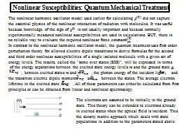
PPT-Nonlinear Susceptibilities: Quantum Mechanical Treatment PowerPoint Presentation

The nonlinear harmonic oscillator model used earlier for calculating 2 did not capture t he essential physics of the nonlinear interaction of radiation with molecules

Upload by giovanna-bartolotta
Published on 2016-07-23

Presentation Embed Code

<iframe width="560" height="315" src="https://www.docslides.com/embed/417187" frameborder="0" allowfullscreen></iframe>

Download Presentation

Download Presentation The PPT/PDF document "Nonlinear Susceptibilities: Quantum Mech..." is the property of its rightful owner. Permission is granted to download and print the materials on this web site for personal, non-commercial use only, and to display it on your personal computer provided you do not modify the materials and that you retain all copyright notices contained in the materials. By downloading content from our website, you accept the terms of this agreement.