PPT-Reduction of Temporal Discretization Error in an Atmospheric General Circulation Model PowerPoint Presentation

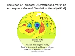
Daisuke Hotta hottaumdedu Advisor Prof Eugenia Kalnay Dept of Atmospheric and Oceanic Science University of Maryland College Park ekalnayatmosumdedu Numerical

Upload by giovanna-bartolotta
Published on 2018-03-12

Presentation Embed Code

<iframe width="560" height="315" src="https://www.docslides.com/embed/648636" frameborder="0" allowfullscreen></iframe>

Download Presentation

Download Presentation The PPT/PDF document "Reduction of Temporal Discretization Err..." is the property of its rightful owner. Permission is granted to download and print the materials on this web site for personal, non-commercial use only, and to display it on your personal computer provided you do not modify the materials and that you retain all copyright notices contained in the materials. By downloading content from our website, you accept the terms of this agreement.