PPT-STT 200 – Lecture 5, section 23,24

Author : giovanna-bartolotta | Published Date : 2016-08-15

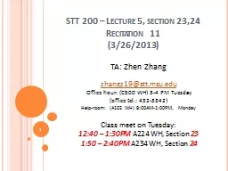
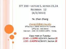
Recitation 12 422013 TA Zhen Zhang zhangz19sttmsuedu Office hour C500 WH 34 PM Tuesday office tel 4323342 Helproom A102 WH 900AM100PM Monday Class meet on

Presentation Embed Code

Download Presentation

Download Presentation The PPT/PDF document "STT 200 – Lecture 5, section 23,24" is the property of its rightful owner. Permission is granted to download and print the materials on this website for personal, non-commercial use only, and to display it on your personal computer provided you do not modify the materials and that you retain all copyright notices contained in the materials. By downloading content from our website, you accept the terms of this agreement.

STT 200 – Lecture 5, section 23,24: Transcript

Recitation 12 422013 TA Zhen Zhang zhangz19sttmsuedu Office hour C500 WH 34 PM Tuesday office tel 4323342 Helproom A102 WH 900AM100PM Monday Class meet on Tuesday . Recitation 13. (11/27/2012). TA: Zhen . (Alan) . Zhang. zhangz19@stt.msu.edu. Office hour: (C500 WH) 1:45 – 2:45PM . Tuesday. (office . tel.: . 432-3342). Help-room: (A102 WH) 11:20AM-12:30PM, . Monday, Friday. The 200 Set: Level of Play. The “200” set is a simple set that is suitable for players of all ages and skill levels. “200” can be used in much the same was “60” and “60 Go” are used, as a set designed to “take the air” out of the ball, slow the pace of the game and give the defense time to rest. For simplicity sake we will only be implementing the “200” at the higher levels.. Today’s Lecture. The Relational Model & Relational Algebra. Relational . Algebra Pt. II . [Optional: may skip]. 2. Lecture 16. 1. The Relational Model & Relational Algebra. 3. Lecture 16 > Section 1. Recitation 13. (4/9/2013). 1. TA: Zhen Zhang. zhangz19@stt.msu.edu. Office hour: (C500 WH) 3-4 PM Tuesday. (. office . tel.: . 432-3342). Help-room: (A102 WH) . 9:00AM-1:00PM. , . Monday. Class meet on Tuesday: . Recitation 14. (12/4/2012). TA: Zhen . (Alan) . Zhang. zhangz19@stt.msu.edu. Office hour: (C500 WH) 1:45 – 2:45PM . Tuesday. (office . tel.: . 432-3342). Help-room: (A102 WH) 11:20AM-12:30PM, . Monday, Friday. Recitation 13. (11/27/2012). TA: Zhen . (Alan) . Zhang. zhangz19@stt.msu.edu. Office hour: (C500 WH) 1:45 – 2:45PM . Tuesday. (office . tel.: . 432-3342). Help-room: (A102 WH) 11:20AM-12:30PM, . Monday, Friday. . - inverse model . components (structure . / data flow. ). - building process (code versioning/sync. .). Model development. . - develop based on v11-02. . - get GCHP to run . backwards (could be trivial). Vectors Math 200 Week 1- Wednesday Math 200 Main Questions for Today What is a vector? What operations can we do with vectors? What kinds of representations and notations do we have for vectors? What are some of the important properties of vectors? STT 200 – Lecture 1, section 2,4 Recitation 11 (11/13/2012) TA: Zhen (Alan) Zhang zhangz19@stt.msu.edu Office hour: (C500 WH) 1:45 – 2:45PM Tuesday (office tel.: 432-3342) Help-room: (A102 WH) 11:20AM-12:30PM, Recitation . 11. (3/26/2013. ). TA: Zhen Zhang. zhangz19@stt.msu.edu. Office hour: (C500 WH) 3-4 PM Tuesday. (. office . tel.: . 432-3342). Help-room: (A102 WH) . 9:00AM-1:00PM. , . Monday. Class meet on Tuesday: . David Chan, MD, PT. Suncoast . Orthopaedic. Surgery & Sports Medicine. Venice, FL. FINANCIAL DISCLOSURES. DISCUSSION GOALS. REVIEW COMMON ARTHRITIS PATTERNS. REVIEW HISTORICAL SURGICAL INTERVENTIONS. FACEBOOK FOLLOWERSANNUALLYBUILDERS ASSOCIATES EMAIL DATABASETO GET STARTEDTo reserve your ad space or to Availability Logo contact information and tagline placement in bottom section of the Availabil for the ANKE-Collaboration. Spin2014 . October . 20, 2014. Initial . Research of . np. Scattering with Polarized Deuterium Target at ANKE/COSY. Hundreds of candidates take the CrowdStrike Certified Falcon Administrator (CCFA) CCFA-200 exam to prove the knowledge and skills. It is highly recommended to use the CrowdStrike CCFA-200 exam questions of Killtest to pass the CrowdStrike Certified Falcon Administrator (CCFA) exam successfully and quickly. Killtest offers the latest CCFA-200 practice exam with actual questions and answers that help you learn the exam well. All our CrowdStrike CCFA-200 exam questions are endorsed by experts. We offer such questions that cover all domains of the CCFA-200 exam. #CrowdStrike CCFA-200 Exam Questions

Download Document

Here is the link to download the presentation.
"STT 200 – Lecture 5, section 23,24"The content belongs to its owner. You may download and print it for personal use, without modification, and keep all copyright notices. By downloading, you agree to these terms.