/
Webinar: What’s  New in SigmaXL Version Webinar: What’s  New in SigmaXL Version

Webinar: What’s New in SigmaXL Version - PowerPoint Presentation

hanah
hanah . @hanah
Follow
0 views
Uploaded On 2024-03-13

Webinar: What’s New in SigmaXL Version - PPT Presentation

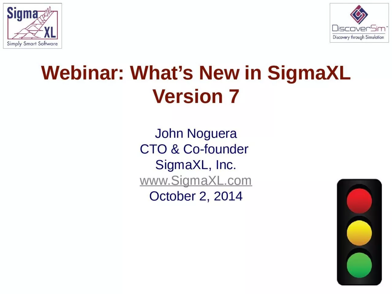
7 John Noguera CTO amp Cofounder SigmaXL Inc wwwSigmaXLcom October 2 2014 2 SigmaXL has added some exciting new and unique features Traffic Light Automatic Assumptions Check for Ttests and ID: 1047859

test sample data exact sample test exact data measurement analysis systems nonparametric report attribute highlighted agreement equal assumptions contingency

Share:

Link:

Embed:

Download Presentation from below link

Download Presentation The PPT/PDF document "Webinar: What’s New in SigmaXL Versio..." is the property of its rightful owner. Permission is granted to download and print the materials on this web site for personal, non-commercial use only, and to display it on your personal computer provided you do not modify the materials and that you retain all copyright notices contained in the materials. By downloading content from our website, you accept the terms of this agreement.


Presentation Transcript

1. Webinar: What’s New in SigmaXL Version 7John NogueraCTO & Co-founder SigmaXL, Inc.www.SigmaXL.comOctober 2, 2014

2. 2SigmaXL has added some exciting, new and unique features:“Traffic Light” Automatic Assumptions Check for T-tests and ANOVAWhat’s New in SigmaXL Version 7A text report with color highlight gives the status of assumptions: Green (OK), Yellow (Warning) and Red (Serious Violation).Normality, Robustness, Outliers, Randomness and Equal Variance are considered.

3. 3“Traffic Light” Attribute Measurement Systems Analysis: Binary, Ordinal and NominalWhat’s New in SigmaXL Version 7A Kappa color highlight is used to aid interpretation: Green (> .9), Yellow (.7-.9) and Red (< .7) for Binary and Nominal. Kendall coefficients are highlighted for Ordinal. A new Effectiveness Report treats each appraisal trial as an opportunity, rather than requiring agreement across all trials.

4. 4Automatic Normality Check for Pearson CorrelationWhat’s New in SigmaXL Version 7A yellow highlight is used to recommend significant Pearson or Spearman correlations. A bivariate normality test is utilized and Pearson is highlighted if the data are bivariate normal, otherwise Spearman is highlighted.

5. 5Small Sample Exact Statistics for One-Way Chi-Square, Two-Way (Contingency) Table and Nonparametric TestsWhat’s New in SigmaXL Version 7Exact statistics are appropriate when the sample size is too small for a Chi-Square or Normal approximation to be valid.For example, a contingency table where more than 20% of the cells have an expected count less than 5.Exact statistics are typically available only in advanced and expensive software packages!

6. 6“Traffic Light” Automatic Assumptions Check for T-tests and ANOVAWhat’s New in SigmaXL Version 7A text report with color highlight gives the status of assumptions: Green (OK), Yellow (Warning) and Red (Serious Violation).Normality, Robustness, Outliers, Randomness and Equal Variance are considered.

7. 7Each sample is tested for Normality using the Anderson-Darling (AD) test. If the AD P-Value is less than 0.05, the cell is highlighted as yellow (i.e., warning – proceed with caution). The Skewness and Kurtosis are reported and a note added, “See robustness and outliers.”If the AD P-Value is greater than or equal to 0.05, the cell is highlighted as green.Hypothesis Test Assumptions Report - Normality

8. 8A minimum sample size for robustness to nonnormality is determined using minimum sample size equations derived from extensive Monte Carlo simulations. Determine a minimum sample size required for a test to be robust, given a specified sample Skewness and Kurtosis.If each sample size is greater than or equal to the minimum for robustness, the minimum sample size value is reported and the test is considered to be robust to the degree of nonnormality present in the sample data:If any sample size is less than the minimum for robustness, the minimum sample size value is reported and a suitable Nonparametric Test is recommended. The cell is highlighted in red:Hypothesis Test Assumptions Report - Robustness

9. 9Each sample is tested for outliers using Tukey’s Boxplot Rules: Potential (> Q3 + 1.5*IQR or < Q1 – 1.5*IQR); Likely: 2*IQR; Extreme: 3*IQR. If outliers are present, a warning is given and recommendation to review the data with a Boxplot and Normal Probability Plot and to consider using a Nonparametric Test.If no outliers are found, the cell is highlighted as green:If a Potential or Likely outlier is found, the cell is highlighted as yellow:Note that upper and lower outliers are distinguished.Hypothesis Test Assumptions Report - Outliers (Boxplot Rules)

10. 10If an Extreme outlier is found, the cell is highlighted as red:The Anderson Darling normality test is applied to the sample data with outliers excluded. If this results in an AD P-Value that is greater than 0.1, a notice is given, “Excluding the outliers, data are inherently normal." The cell remains highlighted as yellow or red.Hypothesis Test Assumptions Report - Outliers (Boxplot Rules)

11. 11Each sample is tested for randomness (serial independence) using the Exact Nonparametric Runs Test. If the sample data is not random, a warning is given and recommendation to review the data with a Run Chart or Control Chart. If the Exact Nonparametric Runs Test P-Value is greater than or equal to 0.05, the cell is highlighted as green.If the Exact Nonparametric Runs Test P-Value is less than 0.05, but greater than or equal to 0.01, the cell is highlighted as yellow.If the Exact Nonparametric Runs Test P-Value is less than 0.01, the cell is highlighted as red.Hypothesis Test Assumptions Report - Randomness

12. 12The test for Equal Variances is applicable for two or more samples. If all sample data are normal, the F-Test (2 sample) or Bartlett’s Test (3 or more samples) is utilized. If any samples are not normal, i.e., have an AD P-Value < .05, Levene’s test is used. If the variances are unequal and the test being used is the equal variance option, then a warning is given and Unequal Variance (2 sample) or Welch’s Test (3 or more samples) is recommended.If the test for Equal Variances P-Value is >= .05, the cell is highlighted as green:Hypothesis Test Assumptions Report – Equal Variance

13. 13If the test for Equal Variances P-Value is >= .05, but the Assume Equal Variances is unchecked (2 sample) or Welch’s ANOVA (3 or more samples) is used, the cell is highlighted as yellow:If the test for Equal Variances P-Value is < .05, and the Assume Equal Variances is checked (2 sample) or regular One-Way ANOVA (3 or more samples) is used, the cell is highlighted as red:Hypothesis Test Assumptions Report – Equal Variance

14. 14If the test for Equal Variances P-Value is < .05, and the Assume Equal Variances is unchecked (2 sample) or Welch’s ANOVA (3 or more samples) is used, the cell is highlighted as green:Hypothesis Test Assumptions Report – Equal Variance

15. 15Open Customer Data.xlsx. Click SigmaXL > Statistical Tools > One-Way ANOVA & Means Matrix. Select variables as shown:Hypothesis Test Assumptions Report – Example: One-Way ANOVA

16. 16Hypothesis Test Assumptions Report – Example: One-Way ANOVA

17. 17Hypothesis Test Assumptions Report – Example: One-Way ANOVASigmaXL > Graphical Tools > Histograms & Descriptive StatisticsSigmaXL > Graphical Tools > Boxplots

18. 18Open Nonnormal Task Time Difference – Small Sample.xlsx.A study was performed to determine the effectiveness of training to reduce the time required to complete a short but repetitive process task. Fifteen operators were randomly selected and the difference in task time was recorded in seconds (after training – before training). A negative value denotes that the operator completed the task in less time after training than before.H0: Mean Difference = 0; Ha: Mean Difference < 0.Hypothesis Test Assumptions Report Example – 1 Sample t-Test with Small Sample Nonnormal DataSigmaXL > Statistical Tools > 1 Sample t-Test & Confidence Intervals.

19. 19Hypothesis Test Assumptions Report Example – Small Sample NonnormalThe recommended One Sample Wilcoxon Exact will be demonstrated later.

20. 20Hypothesis Test Assumptions Report Example – Small Sample NonnormalSigmaXL > Graphical Tools > Histograms & Descriptive Statistics.This small sample data fails the Anderson Darling Normality Test (P-Value = .023). Note that this is due to the data being uniform or possibly bimodal, not due to a skewed distribution.

21. 21“Traffic Light” Attribute Measurement Systems Analysis: Binary, Ordinal and NominalWhat’s New in SigmaXL Version 7A Kappa color highlight is used to aid interpretation: Green (> .9), Yellow (.7-.9) and Red (< .7) for Binary and Nominal. Kendall coefficients are highlighted for Ordinal. A new Effectiveness Report treats each appraisal trial as an opportunity, rather than requiring agreement across all trials.

22. 22Confidence intervals for binomial proportions have an "oscillation" phenomenon where the coverage probability varies with n and p. Exact (Clopper-Pearson) is strictly conservative and will guarantee the specified confidence level as a minimum coverage probability, but results in wide intervals. This is recommended only for applications requiring strictly conservative intervals. Wilson Score has mean coverage probability matching the specified confidence interval. Since the Wilson Score intervals are narrower and thereby more powerful, they are recommended for use in Attribute MSA studies due to the small sample sizes typically used [1, 2, 3].Attribute Measurement Systems Analysis: Percent Confidence Intervals (Exact or Wilson Score)

23. 23The Attribute Effectiveness Report is similar to the Attribute Agreement Report, but treats each trial as an opportunity. Consistency across trials or appraisers is not considered. This has the benefit of providing a Percent measure that is unaffected by the number of trials or appraisers. The increased sample size for # Inspected results in a reduction of the width of the Percent confidence interval. The Misclassification report shows all errors classified as Type I or Type II. Mixed errors are not relevant here. This report requires a known reference standard and includes: Each Appraiser vs. Standard Effectiveness, All Appraisers vs. Standard Effectiveness, and Effectiveness and Misclassification Summary.Attribute Measurement Systems Analysis: Effectiveness Report

24. 24Kappa can vary from -1 to +1, with +1 implying complete consistency or perfect agreement between assessors, zero implying no more consistency between assessors than would be expected by chance and -1 implying perfect disagreement.Fleiss [4] gives the following rule of thumb for interpretation of Kappa:Kappa: >= 0.75 signifies excellent agreement, for most purposes, and <= 0.40 signifies poor agreement.AIAG recommends the Fleiss guidelines [5].Attribute Measurement Systems Analysis: Kappa Interpretation

25. 25In Six Sigma process improvement applications, a more rigorous level of agreement is commonly used. Futrell [6] recommends:The lower limit for an acceptable Kappa value (or any other reliability coefficient) varies depending on many factors, but as a general rule, if it is lower than 0.7, the measurement system needs attention. The problems are almost always caused by either an ambiguous operational definition or a poorly trained rater. Reliability coefficients above 0.9 are considered excellent, and there is rarely a need to try to improve beyond this level.Attribute Measurement Systems Analysis: Kappa Interpretation

26. 26SigmaXL uses the guidelines given by Futrell and color codes Kappa as follows: >= 0.9 is green, 0.7 to 0.9 is yellow and < 0.7 is red. This is supported by the following relationship to Spearman Rank correlation and Percent Effectiveness/Agreement (applicable when the response is binary with an equal proportion of good and bad parts):Kappa = 0.7; Spearman Rank Correlation = 0.7; Percent Effectiveness = 85%; Percent Agreement = 85% (two trials)Kappa = 0.9; Spearman Rank Correlation = 0.9; Percent Effectiveness = 95%; Percent Agreement = 95% (two trials)Note that these relationships do not hold if there are more than two response levels or the reference proportion is different than 0.5. Attribute Measurement Systems Analysis: Kappa Interpretation

27. 27Kendall's Coefficient of Concordance (Kendall's W) is a measure of association for discrete ordinal data, typically used for assessments that do not include a known reference standard. Kendall’s coefficient of concordance ranges from 0 to 1: A coefficient value of 1 indicates perfect agreement. If the coefficient is low, then agreement is random, i.e., the same as would be expected by chance. Attribute Measurement Systems Analysis: Kendall’s Coefficient of Concordance - Interpretation

28. 28There is a close relationship between Kendall’s W and Spearman’s (mean pairwise) correlation coefficient [7]:Confidence limits for Kendall’s Concordance cannot be solved analytically, so are estimated using bootstrapping.Ruscio [8] demonstrates the bootstrap for Spearman’s correlation and we apply this method to Kendall’s Concordance. The data are row wise randomly sampled with replacement to provide the bootstrap sample (N = 2000). W can be derived immediately from the mean value of the Spearman’s correlation matrix from the bootstrap sample.Attribute Measurement Systems Analysis: Kendall’s Coefficient of Concordance - Interpretationk is the number of trials (within) or trials*appraisers (between)

29. 29SigmaXL uses the following “rule-of-thumb” interpretation guidelines: >= 0.9 very good agreement (color coded green)0.7 to < 0.9 marginally acceptable, improvement should be considered (yellow)< 0.7 unacceptable (red). This is consistent with Kappa and is supported by the relationship to Spearman’s correlation.Note, however, that in the case of Within Appraiser agreement with only two trials, the rules should be adjusted: very good agreement is >= 0.95unacceptable agreement is < 0.85. Attribute Measurement Systems Analysis: Kendall’s Coefficient of Concordance - Interpretation

30. 30Kendall's Correlation Coefficient (Kendall's tau-b) is a measure of association for discrete ordinal data, used for assessments that include a known reference standard.Kendall’s correlation coefficient ranges from -1 to 1: A coefficient value of 1 indicates perfect agreement. If coefficient = 0, then agreement is random, i.e., the same as would be expected by chance. A coefficient value of -1 indicates perfect disagreement.Kendall's Correlation Coefficient is a measure of rank correlation, similar to the Spearman rank coefficient, but uses concordant (same direction) and discordant pairs [10].Attribute Measurement Systems Analysis: Kendall’s Correlation Coefficient - Interpretation

31. 31SigmaXL uses the following “rule-of-thumb” interpretation guidelines: >= 0.8 very good agreement (color coded green);0.6 to < 0.8 marginally acceptable, improvement should be considered (yellow);< 0.6 unacceptable (red).These values were determined using Monte Carlo simulation with correlated integer uniform distributions. They correspond approximately to Spearman 0.7 and 0.9 when there are 5 ordinal response levels (1 to 5). With 3 response levels, the rule-of-thumb thresholds should be modified to 0.65 and 0.9.Attribute Measurement Systems Analysis: Kendall’s Correlation Coefficient - Interpretation

32. 32Open the file Attribute MSA – AIAG.xlsx. This is an example from the Automotive Industry Action Group (AIAG) MSA Reference Manual, 3rd edition, page 127 (4th Edition, page 134). There are 50 samples, 3 appraisers and 3 trials with a 0/1 response. A “good” sample is denoted as a 1. A “bad” sample is denoted as a 0. Attribute Measurement Systems Analysis – Binary ExampleSigmaXL > Measurement Systems Analysis > Attribute MSA (Binary)

33. 33Attribute Measurement Systems Analysis – Binary Example

34. 34Attribute Measurement Systems Analysis – Binary Example

35. 35Attribute Measurement Systems Analysis – Binary Example

36. 36Attribute Measurement Systems Analysis – Binary Example

37. 37Open the file Attribute MSA – Ordinal.xlsx. This is an Ordinal MSA example with 50 samples, 3 appraisers and 3 trials. The response is 1 to 5, grading product quality. One denotes “Very Poor Quality,” 2 is “Poor,” 3 is “Fair,” 4 is “Good” and a 5 is “Very Good Quality.” The Expert Reference column is the reference standard from an expert appraisal. Attribute Measurement Systems Analysis – Ordinal ExampleSigmaXL > Measurement Systems Analysis > Attribute MSA (Ordinal)

38. 38Attribute Measurement Systems Analysis – Ordinal Example

39. 39Attribute Measurement Systems Analysis – Ordinal Example

40. 40Attribute Measurement Systems Analysis – Ordinal Example

41. 41An automatic normality check is applied to pairwise correlations in the correlation matrix, utilizing the powerful Doornik-Hansen bivariate normality test. A yellow highlight recommends Pearson or Spearman correlations be used (but only if it is significant). Pearson is highlighted if the data are bivariate normal, otherwise Spearman is highlighted. Always review the data graphically with scatterplots as well.Automatic Normality Check for Pearson Correlation

42. 42Small Sample Exact Statistics for One-Way Chi-Square, Two-Way (Contingency) Table and Nonparametric TestsWhat’s New in SigmaXL Version 7Exact statistics are appropriate when the sample size is too small for a Chi-Square or Normal approximation to be valid.For example, a contingency table where more than 20% of the cells have an expected count less than 5.Exact statistics are typically available only in advanced and expensive software packages!

43. 43Nonparametric tests do not assume that the sample data are normally distributed, but they do assume that the test statistic follows a Normal or Chi-Square distribution when computing the “large sample” or “asymptotic” p-value. The One-Sample Sign Test, Wilcoxon Signed Rank, Two Sample Mann-Whitney and Runs Test assume a Normal approximation for the test statistic. Kruskal-Wallis and Mood’s Median use Chi-Square to compute the p-value. With very small sample sizes, these approximations may be invalid, so exact methods should be used. SigmaXL computes the exact P-Values utilizing permutations and fast network algorithms.Exact Nonparametric Tests

44. 44It is important to note that while exact p-values are “correct,” they do not increase (or decrease) the power of a small sample test, so they are not a solution to the problem of failure to detect a change due to inadequate sample size.Exact Nonparametric Tests

45. 45For data that require more computation time than specified, Monte Carlo P-Values provide an approximate (but unbiased) p-value that typically matches exact to two decimal places using 10,000 replications. One million replications give a P-Value that is typically accurate to three decimal places. A confidence interval (99% default) is given for the Monte Carlo P-Values. Note that the Monte Carlo confidence interval for P-Value is not the same as a confidence interval on the test statistic due to data sampling error. The 99% Monte Carlo P-Value confidence interval is due to the uncertainty in Monte Carlo sampling, and it becomes smaller as the number of replications increases (irrespective of the data sample size). The Exact P-Value will lie within the stated Monte Carlo confidence interval 99% of the time.Exact Nonparametric Tests – Monte Carlo

46. 46Sign Test: N <= 50Wilcoxon Signed Rank: N <= 15Mann-Whitney: Each sample N <= 10Kruskal-Wallis: Each sample N <= 5Mood’s Median: Each sample N <= 10Runs Test (Above/Below) or Runs Test (Up/Down) Test: N <= 50These are sample size guidelines for when exact nonparametric tests should be used rather than “large sample” asymptotic based on the Normal or Chi-Square approximation. It is always acceptable to use an exact test, but computation time can become an issue especially for tests with two or more samples. In those cases, one can always use a Monte Carlo P-Value with 99% confidence interval.Exact Nonparametric Tests - Recommended Sample Sizes

47. 47If more than 20% of the cells have expected counts less than 5 (or if any of the cells have an expected count less than 1), the Chi-Square approximation may be invalid. Fisher’s Exact utilizes permutations and fast network algorithms to solve the Exact Fisher P-Value for contingency (two-way row*column) tables. This is an extension of the Fisher Exact option provided in the Two Proportion Test template. For data that requires more computation time than specified, Monte Carlo P-Values provide an approximate (but unbiased) p-value.Fisher’s Exact for Two Way Contingency Tables

48. 48The Chi-Square statistic requires that no more than 20% of cells have an expected count less than 5 (and none of the cells have an expected count less than 1). If this assumption is not satisfied, the Chi-Square approximation may be invalid and Exact or Monte Carlo P-Values should be used. Chi-Square Exact solves the permutation problem using enhanced enumeration.Exact One-Way Chi-Square Goodness of Fit

49. 49See SigmaXL Workbook Appendix: Exact and Monte Carlo P-Values for Nonparametric and Contingency Test.Exact and Monte Carlo P-Valuesfor Nonparametric and Contingency Tests

50. 50Open the file Nonnormal Task Time Difference – Small Sample.xlsx. Earlier we performed a 1 Sample t-Test on the task time difference data for effectiveness of training. The Assumptions Report recommended the One Sample Wilcoxon – Exact.H0: Mean Difference = 0; Ha: Mean Difference < 0.One Sample Wilcoxon Exact – ExampleSigmaXL > Statistical Tools > Nonparametric Tests – Exact > 1 Sample Wilcoxon - ExactReject H0.

51. 51One Sample Wilcoxon Exact – ExampleSigmaXL > Statistical Tools > Nonparametric Tests > 1 Sample WilcoxonThis is the large sample (asymptotic) Wilcoxon TestIncorrectly failed to reject H0 (Type II). Note that the error could have gone in the other direction (Type I), or large sample could have agreed with exact. The problem with using a large sample test with small sample data is the uncertainty of the p-value!

52. 52Open the file Oral_Lesions.xlsx. We will consider a sparse data set where the Chi-Square approximation fails and Fisher’s Exact is required to give a correct conclusion for the hypothesis test.This is adapted from a subset of dental health data (oral lesions) obtained from house to house surveys that were conducted in three geographic regions of rural India [1, 2]. The Fisher’s Exact P-Value obtained with SigmaXL may be validated using these references. The data labels have been modified to a generic “A”, “B”, “C”, etc. for the oral lesions location (rows) and “Region1”, “Region2” and “Region3” for the geographic regions (columns).Fisher’s Exact for Two Way Contingency Tables – Example

53. 53Fisher’s Exact for Two Way Contingency Tables – ExampleSigmaXL > Statistical Tools > Chi-Square Tests – Exact > Chi-Square Test – Two-Way Table Data – Fisher’s Exact

54. 54Fisher’s Exact for Two Way Contingency Tables – ExampleLarge sample (asymptotic) Chi-Square incorrectly failed to reject H0.Fisher’s Exact rejects H0.

55. 55Fisher’s Exact for Two Way Contingency Tables – ExamplePress F3 or click Recall SigmaXL Dialog to recall last dialog

56. 56Fisher’s Exact for Two Way Contingency Tables – Example

57. Webinar: What’s New in SigmaXL Version 7Questions?

58. 58Agresti, A. and Coull, B.A.(1998). “Approximate is Better than “Exact” for Interval Estimation of Binomial Proportions.” The American Statistician, 52, 119–126. Clopper, C.J.,and Pearson, E.S.(1934). “The Use of Confidence or Fiducial Limits Illustrated in the Case of the Binomial.” Biometrika, 26, 404–413. Newcombe, R. (1998a). “Two-sided confidence intervals for the single proportion: Comparison of seven methods.” Statistics in Medicine,17, 857-872.Fleiss, J.L. (2003). Statistical Methods for Rates and Proportions, 3rd Edition., Wiley & Sons, NY.Attribute Measurement Systems Analysis: References

59. 59Automotive Industry Action Group AIAG (2010). Measurement Systems Analysis MSA Reference Manual, 4th Edition, p. 137.Futrell, D. (May 1995). “When Quality Is a Matter of Taste, Use Reliability Indexes,” Quality Progress,81-86.Siegel, S., & Castellan, N.J. (1988). Nonparametric statistics for the behavioral sciences (2nd Ed.). New York, NY: McGraw-Hill. p. 262.Ruscio, J. (2008). “Constructing Confidence Intervals for Spearman’s Rank Correlation with Ordinal Data: A Simulation Study Comparing Analytic and Bootstrap Methods,” Journal of Modern Applied Statistical Methods, Vol. 7, No. 2, 416-434.Bradley Efron, (1987). “Better bootstrap confidence intervals (with discussion),” J. Amer. Statist. Assoc. Vol. 82, 171-200.http://en.wikipedia.org/wiki/Kendall_tau_rank_correlation_coefficientAttribute Measurement Systems Analysis: References

60. 60Doornik, J.A. and Hansen, H. “An Omnibus Test for Univariate and Multivariate Normality,” Oxford Bulletin Of Economics And Statistics, 70, Supplement (2008).Pearson Bivariate Normality Test Reference

61. 61Cyrus R. Mehta & Nitin R. Patel. (1983). "A network algorithm for performing Fisher's exact test in r x c contingency tables." Journal of the American Statistical Association, Vol. 78, pp. 427-434.Siegel, S., & Castellan, N.J. (1988). Nonparametric Statistics for the Behavioral Sciences (2nd Ed.). New York, NY: McGraw-Hill.Gibbons, J.D. and Chakraborti, S. (2010). Nonparametric Statistical Inference (5th Edition). New York: Chapman & Hall.Yates, D., Moore, D., McCabe, G. (1999). The Practice of Statistics (1st Ed.). New York: W.H. Freeman. Cochran WG. “Some methods for strengthening the common [chi-squared] tests.” Biometrics 1954; 10:417–451. Mehta, C. R.; Patel, N. R. (1997) "Exact inference in categorical data," unpublished preprint, http://www.cytel.com/Papers/sxpaper.pdf. See Table 7 (p. 33) for validation of Fisher’s Exact p-value.Exact and Monte Carlo P-Values for Nonparametric and Contingency Tests: References

62. 62Mehta, C.R. ; Patel, N.R. (1998). "Exact Inference for Categorical Data." In P. Armitage and T. Colton, eds., Encyclopedia of Biostatistics, Chichester: John Wiley, pp. 1411–1422.Mehta, C.R. ; Patel, N.R. (1986). “A Hybrid Algorithm for Fisher's Exact Test in Unordered rxc Contingency Tables,” Communications in Statistics - Theory and Methods, 15:2, 387-403.Narayanan, A. and Watts, D. “Exact Methods in the NPAR1WAY Procedure,” SAS Institute Inc., Cary, NC.Myles Hollander and Douglas A. Wolfe (1973), Nonparametric Statistical Methods. New York: John Wiley & Sons. https://onlinecourses.science.psu.edu/stat414/node/330Eugene S. Edgington, (1961). “Probability Table for Number of Runs of Signs of First Differences in Ordered Series,” Journal of the American Statistical Association, Vol. 56, pp. 156-159.Exact and Monte Carlo P-Values for Nonparametric and Contingency Tests: References

63. 63David F. Bauer (1972), “Constructing confidence sets using rank statistics,” Journal of the American Statistical Association Vol 67, pp. 687–690.Hongsuk Jorn & Jerome Klotz (2002). “Exact Distribution of the K Sample Mood and Brown Median Test,” Journal of Nonparametric Statistics, 14:3, 249-257.Exact and Monte Carlo P-Values for Nonparametric and Contingency Tests: References