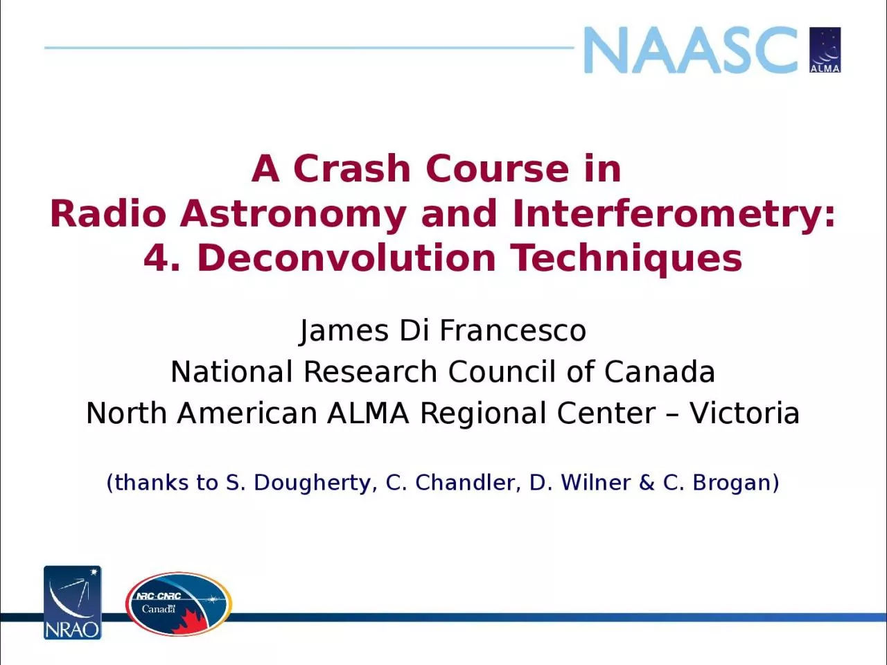
A Crash Course in Radio - PowerPoint Presentation

1. A Crash Course in Radio Astronomy and Interferometry:4. Deconvolution TechniquesJames Di FrancescoNational Research Council of CanadaNorth American ALMA Regional Center – Victoria(thanks to S. Dougherty, C. Chandler, D. Wilner & C. Brogan)

2. difficult to do science on dirty imagedeconvolve b(x,y) from ID(x,y) to recover I(x,y)information is missing, so be careful! (there’s noise, too)dirty image “CLEAN” imageDeconvolutionDeconvolution

3. Deconvolution: uses non-linear techniques effectively interpolate/extrapolate samples of V(u,v) into unsampled regions of the (u,v) planeaims to find a sensible model of I(x,y) compatible with datarequires a priori assumptions about I(x,y)CLEAN (Högbom 1974) is most common algorithm in radio astronomya priori assumption: I(x,y) is a collection of point sourcesvariants for computational efficiency, extended structuredeconvolution requires knowledge of beam shape and image noise properties (usually OK for aperture synthesis)atmospheric seeing can modify effective beam shapedeconvolution process can modify image noise propertiesDeconvolution AlgorithmsDeconvolution

4. Initializea residual map to the dirty mapa CLEAN component listIdentify strongest feature in residual map as a point sourceAdd a fraction g (the loop gain) of this point source to the clean component list (g ~ 0.05-0.3)Subtract the fraction g times b(x,y) from residual mapIf stopping criteria* not reached, go back to step 2 (an iteration), or…Convolve CLEAN component (cc) list with an estimate of the main dirty beam lobe (i.e., the “CLEAN beam”) and add residual map to make the final “restored” imageb(x,y)ID(x,y)Basic CLEAN AlgorithmI(x,y)Deconvolution* Stopping criteria = N x rms (if noise limited), or Imax/N (if dynamic range limited), where N is some arbitrarily chosen value

5. restored imageresidual mapCLEAN modelID(x,y)CLEANDeconvolution

6. CLEAN beam size:natural choice is to fit the central peak of the dirty beam with elliptical Gaussian unit of deconvolved map is Jy per CLEAN beam area (= intensity, can convert to brightness temperature)minimize unit problems when adding dirty map residualsmodest super resolution often OK, but be carefulphotometry should be done with cautionCLEAN does not conserve flux (extrapolates)extended structure missed, attenuated, distortedphase errors (e.g. seeing) can spread signal around “Restored” ImagesDeconvolution

7. “dynamic range”ratio of peak brightness to rms noise in a region void of emission (common in astronomy)an easy to calculate lower limit to the error in brightness in a non-empty region“fidelity”difference between any produced image and the correct imagea convenient measure of how accurately it is possible to make an image that reproduces the brightness distribution on the skyneed a priori knowledge of correct image to calculatefidelity image = input model / difference fidelity is the inverse of the relative errorMeasures of Image QualityDeconvolution

8. Radio Telescopes are coolSingle-dish telescopes measure “temperatures” across the skyThey have fat beams making details hard to seeInterferometers use optics to achieve high resolutionAntenna pairs sample the FT of the image plane, an inverse FT of the ensemble of visibilities returns the imageResulting images are spatially filtered; only compact emission seen“Dirty” images can be deconvolved (with care), e.g., CLEANWeighting can be used to manipulate resolution and/or surface brightness sensitivityMosaics can be used to increase field-of-view but can be observationally expensiveSummary