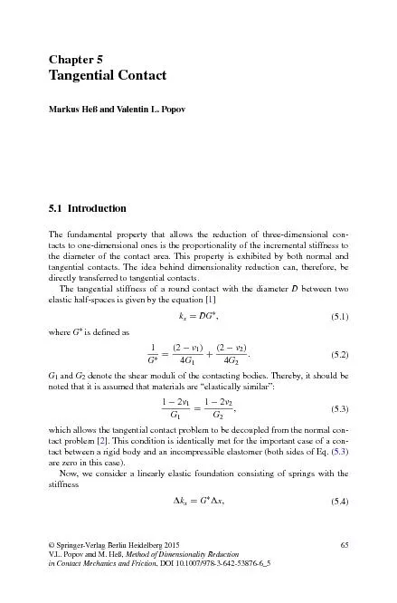
IntroductionThe fundamental property that allows the reduction of thre - PDF document

IntroductionThe fundamental property that allows the reduction of three-dimensional contacts to one-dimensional ones is the proportionality of the incremental stiffness to the diameter of the contact area. This property is exhibited by both normal and tangential contacts. The idea behind dimensionality reduction can, therefore, be The tangential stiffness of a round contact with the diameter between two elastic half-spaces is given by the equation [  is dened as  and denote the shear moduli of the contacting bodies. Thereby, it should be which allows the tangential contact problem to be decoupled from the normal conws the tangential contact problem to be decoupled from the normal con2]. This condition is identically met for the important case of a contact between a rigid body and an incompressible elastomer (both sides of Eq.  (5.2)        (5.3)     (5.4)  Tangential Contact© Springer-Verlag Berlin Heidelberg 2015V.L. Popov and M. Heß, in Contact Mechanics and FrictionMarkus Heß and Valentin L. Popov Tangential Contact  is the distance between the springs. The stiffness () is trivially reproduced with this foundation. In this chapter, we will show that the one-dimensional elastic foundation with the normal stiffness dened in Chap.stiffness (exactlyarbitrarily axially-symmetric proles. We begin our considerations Tangential Contact with Friction for Parabolic BodiesWe consider a rigid three-dimensional parabolic body with the radius of curvature  that is pressed into an elastic half-space with the normal force  quently loaded in the horizontal direction with the force  . We assume that the frictional forces acting in the contact can be simply described using Coulomb’s law of friction with a constant coefcient of friction  dimensional contact problems, it is known that even the application of an arbitrararbitrar1]. With increasing tangential force, the stick domain shrinks until slip is initiated in the entire contact area. In this section, we investigate the one-dimensional mapping of the aforementioned  . The vertical displacement of a spring at a distance  from the middle point of the contact isThe radius  must be set to  method. The elastic force of a single spring at the point  isThe contact radius is obtained from the condition  :(5.5)         (5.6)            (5.7)    Fig. R1 d z FxFN 67 Until now, we have only used the results known from Chap.. Now, we denote the  . Then, the horizontal component of the force acting on a sticking spring isWe determine the boundary of the sticking domain  the tangential force achieves its maximum value:From this, it follows that  1].The slip condition outside of the sticking domain means that every point here fullls Coulomb’s law of friction:Now, we calculate the normal and tangential forces acting in the entire contact area. For the normal force, we once again obtain the Hertzian result:  (5.9)  (5.10)               (5.11)             (5.12)                    (5.13)  (5.14)           (5.15)              (5.16)        Tangential Contact with Friction for Parabolic Bodies Tangential ContactThis result also agrees exactly with that of the three-dimensional problem [We obtain the displacement above which the entire contact area exhibits slip by  which, of course, also agrees exactly with that of the three-dimensional case. Tangential Contact with Friction for Arbitrary In the last section, it was proven that the tangential contact with partial slip for two parabolic bodies can be exactly mapped using the method of dimensionality reduction. The generalization to tangential contacts of arbitrarily formed, axially-symmetric bodies is the topic of this chapter; the complete proofs including all In order to solve the classical three-dimensional contact problem, Cattaneo [[4] initially calculated the tangential displacement in the direction of the applied tangential force, which results from the state of full slip. Subsequently, they superimposed the corresponding tangential stress distribution with a second one of the same form, but with the opposite direction. In this way, constant tan slip. Although the way was paved to solve tangential contact problems with the method of Cattaneo and Mindlin, its application to other geometries appeared exceedingly difcult, because they required explicit knowledge/calculation of the tangential displaceyears later did Truman et al. [cessfully derive the solution to the tangential contact problem between a conical indenter and an elastic half-space. In the same year, Jäger [] arrived at the conclusion that within the framework of Cattaneo-Mindlin theory, every axially-symmetric tangential contact problem can be completely described by the normal contact problem so that an explicit calculation of the tangential displacement is unnecessary. Thereby, we remember that elastically similar materials () are assumed everywhere in this chapter, which allows the contact problem to be decoupled. Furthermore, it is assumed that the frictional stresses point in the direction of the applied tangential force, which strictly speaking, violates a part of Coulomb’s law of friction. Due to the addition of a slippage component perpendicular to the applied force, the tangential stresses and slip are not opposite each other at every point in the slip domain. In [], as well as Chap., it is explained why we can neglect this deviation.           69 6, 9], the tangential stresses are equivalent to the difference between the actual normal stress and those that cient of friction. The same is true for the tangential force  and the relative tan  It is proven in Chap. that based on the Eqs.), these relationships can be obtained from the method of dimensionality reduction. Thus, the method already introduced within the framework of the tangential contact for a parabolic body is generally valid. It consists primarily of two central ansätze:In the one-dimensional equivalent model, the tangential spring forces at the boundary of the stick domain must assume the maximum possible value for the For a given tangential displacement  , the radius of the stick domain  The tangential force is given analogously to the normal force from the sum of the tangential spring forces and, therewith, the tangential distributed loadOn the right side, the piecewise-dened functionAlso, based on the superposition from Jäger, the three-dimensional tangential contact with partial slip can be replaced by two three-dimensional normal contacts. This technique has already been used in various numerical simulations. It is directly evident that such a superposition also retains its validity for the equivalent one-dimensional normal contact. Nevertheless, it is preferred, and requires less effort, to directly map the three-dimensional partial slip problem to a              (5.19)  (5.20)           (5.21)  (5.22)        (5.23)             Tangential Contact with Friction for Arbitrary … Tangential Contactone-dimensional partial slip problem, rather than mapping two three-dimensional Now, we consider an axially-symmetric indenter which has a prole with a form given by a power function with a positive real exponent  sequently, maintaining the normal force, loaded with the tangential force  . We are now looking for the radius of the stick domain and the relative tangential  of both bodies. For the normal contact, one can take the solutions Let us remember that the relationships above arise from the indentation of the which is vertically scaled by the factor  The extension to the tangential contact requires that the spring elements be independent from one another in the tangential direction and possess the stiff  . As in the three-dimensional contact problem, Coulomb’s law of friction is also locally valid in the one-dimensional model. By the addition of a tangential force, the tangential springs in the area near the edge of the contact area  ) slide because the vertical spring forces, and therefore, the maximum  this domain, the spring forces (normal and tangential) at every point are directly  . Within this radius (  tangential spring elements stick and, therefore, experience the same tangential dis  . In summary, the distribution of the tangential spring forces can be expressed by means of the piecewise dened distributed loadWe determine the tangential displacement  as a function of the radius of the stick domain c from the condition ((5.24)  (5.25)  (5.26)       (5.27)  (5.28)            (5.29)                 71 ) provides when taking (For  , the result of the classical contact problem from Cattaneo and Mindlin is obtained, but also the special case of a at, cylindrical indenter can be obtained  . As long as the tangential force  is smaller than the maximum static force of friction  entirein this case. However, if this limit is reached, then complete sliding initiates. shows Eq.) graphically for the above named geometries (parabo  ). The gray curve is for an exponent of  and signies the family of curves for increasing Using the now known radius of stick, one can also determine the tangential displacement with respect to the input values. After inserting (), it follows thatNaturally, Eq.  1]. For the tangential contact between a at, cylindrical indenter and a half-space, the limit  as  must once again be found, which leads to the elementary result of              (5.31)          (5.32)             (5.33)       Fig.  cylindrical indenter Tangential Contact with Friction for Arbitrary … Tangential ContactThe direct proportionality between force and displacement is shown in Fig.The slope triangle on the curve for the at, cylindrical indenter indicates the compliance. For extremely small tangential forces, for which the slip domain is constrained to a very small ring, Eq.) is valid for all proles, regardless of the form function exponent.) allow for the exact mapping of tangential contacts for arbitrarypiecewise dened are also included here. The latter, however, can cause scaling, but must be found by integration (see Problem 3). Mapping of Stresses in the Tangential ContactDue to the principle of superposition from Jäger, the tangential stresses can be obtained, completely analogously to the normal stresses, from the Abel-like integral transformation of the tangential distributed load  . It follows from the alternate presentation of the piecewise-dened, linear force density from () as the difference between two vertical distributed loads and subsequent use of (As an example, we want to use Eq.) on the classical tangential contact between a parabolic body and a plane. In the rst step, we dene the tangential                         Fig. Tangential  plotted with respect to the tangential force  (normalized) 73 linear load for the one-dimensional model, which we already implicitly drew upon In order to keep the effort required to a minimum, we use the integral expression which requires the derivative of the linear load:), we must differentiate between the two cases  and  After simple integration, we obtain  is the Heaviside step function. It is generally known that Eq.corresponds to the exact distribution of the tangential stress in a three-dimensional ution of the tangential stress in a three-dimensional 1].5.5þÿ &#x/Act;&#xualT;xt0;&#x/Act;&#xualT;xt0;  . This denotes the tangential relative displacement of the surface points in the slip domain of the contact area, which is required for the calculation of wear and other tribological processes. For the sake of clarity, the constant tangential displacement of all points within the sticking domain will be denoted in           Let it be noted that in special cases of non-differentiable form functions, only the rst integral expression in (        (5.37)                       (5.38)                       (5.39)  Mapping of Stresses in the Tangential Contact Tangential ContactThe fact that this displacement can be mapped exactly by the method of dimensional reduction has already been shown. In a similar way, the local slip in the slip Once again, Jäger’s principle of superposition is at the center of our considerations. Using this, the following equation for the slip of an axially-symmetric con  can be easily understood:Here,  is the tangential displacement of the surface of the linearly elastic For the classical tangential contact of a parabolic body with a plane, the appli) will be explained in the following. For this, we rst introduce slip in the one-dimensional model. From the tangential distributed equivalent system. This is because both are proportional to each other, whereby the effective shear modulus  is the proportionality factor:With this, the following is valid for the one-dimensional slip:  (5.41)           (5.42)              (5.43)              (5.44)                   (5.45)                   75 ProblemsProblem 1Determine the radius of stick and the relative tangential displacement with respect to the tangential force for the tangential contact between an elastic assumed that the normal contact problem for which tangential loading is investigated has already been solved (see Problem 1 in Chap.The equivalent one-dimensional contact problem consists of a rigid cross-section of a conical indenter scaled vertically by a factor of  quently loaded with a tangential force. All tangential spring elements whose spring forces have not yet reached the spatially-dependent maximum static force of fric  undergo the respective displacement  . In the outer ring, the vertical ing occurs. At the stick–slip limit, the tangential spring forces must assume the  ) can be brought into the following form:              (5.47)                  (5.48)                     (5.49)       (5.50)          5.6 Tangential Contact  spond exactly with the three-dimensional solution from Truman et al. [Problem 2Calculate the tangential stress distribution within the contact area for the tangential contact handled in Problem 1 with the help of the Abel transformadimensional model requires setting up the equation for and subsequently differentiating the tangential linear load. The linear load was already implicitly used to ). Its derivative is) initially providesand after integration and simple rearrangement,The tangential stress distribution, normalized by the mean value in the case of for sizes of the stick domain. The nite value at the point  is(5.51)        (5.52)                       (5.53)                       (5.54)                                    Fig. tangential stress distribution    77 Problem 3 A at, cylindrical indenter with rounded edges is initially pressed into an elastic half-space with the normal force   and subsequently loaded with a (presently unknown) tangential force   , which results in a given relative tangen - tial displacement   of the two bodies. It is assumed that the bodies are composed of elastically similar materials and that the prole of the indenter is given by the following (see Fig. 5.5 ): Determine the indentation depth and normal force as a function of contact radius with the help of the reduction method. Furthermore, calculate the tangential dis - placement and tangential force as a function of the stick radius. Solution In the rst step, the one-dimensional equivalent prole must be deter - mined. The piecewise-dened function according to ( 5.55 ) requires the application of the generalized formula (3.27) Calculating the integral in Eq. ( 5.56 ) requires nothing more than elementary mathematics: Nevertheless, we must remember that ( 5.56 ) has to be extended axis-symmetri - cally to the domain of       . Then, we obtain The normalized original and equivalent proles are shown in Fig. 5.6 . (5.55)                            (5.56)                                                       (5.57)                             (5.58)                                                Fig. 5.5 Tangential contact of a at indenter with rounded edges (radius R ) 5.6 Problems Tangential ContactIntegration, taking (  is a parabolic prole. As expected, the Eqs.words, requiring that the tangential spring force reaches the maximum possible  . With the help of (                (5.60)               (5.61)                          (5.62)                           Fig. 79 Now, it is only left to nd the dependence between the tangential force and the stick radius. For this, we look at a distributed load in the one-dimensional modeland integrate this over the contact width in the reduced model:The integral on the right-hand side already appeared in the calculation of the normal force in (). After calculating the antiderivative and taking the lower limit of integration into account, we obtainWe can be directly convinced of the correctness of Eq.) if we consider the principle of superposition by Jäger. According to (equivalent to the difference between the current normal force and one that would this relationship can be easily veried. Figure shows the normalized dependence of the stick radius on the tangential force for various cases. The limiting case  if the contact area is only slightly larger than the at section (  curve approaches that of a at indenter. A comparison is shown in Fig.                  (5.64)                (5.65)                     Fig.  for a at indenter with rounded edges 5.6 Tangential ContactAlthough it has not yet been mentioned, it was assumed in the above calculations that  , and therefore, partial sliding within the at section is not possible. Figure emphasizes the validity of this assumption. As soon as the slip domain includes the rounded edges, then the transition to complete slip takes place. For the analogous planar contact problem, a corresponding behavior was analytically proven [] and veried by nite element calculations [Problem 4Determine the integral form for the normal and tangential stress distribution for the contact between a at indenter with rounded edges having a radius of curvature of ). Assume a constant distributed loading of the one-dimensional model and visualize the numeric solutions of the integral expressions.The vertical distributed load in the one-dimensional model is directly proportional to the normal displacement of the surface and according to Eq.The derivative is required for the calculation of the normal stress distribution. Because of axial symmetry, we only have to determine this for positive These integral relations are identical to those of the three-dimensional theory. They must be solved numerically. Figure shows the distribution of the normal  is the mean stress. Several ratios are shown. For  , we understandably obtain the Hertzian results, while for  larity at the edges of the contact for a at, cylindrical indenter (with sharp edges).  towards the center.The calculation of the tangential stress follows completely analogously. The tangential distributed load of the linearly elastic foundation was already shown in Problem 3 so that we must now only focus on  and differentiate (               (5.67)                         (5.68)                           (5.69)                          81 ) results in the distribution of the tangential stress in integral form, which corresponds to () with the exception of the integral values  . A comparison with Fig. allows the principle of superposi  and the arbitrarily chosen ratio of stick to contact radius  Mindlin is evident.                     Fig. Distribution of cases shown are those from  pressure distribution) as well  Fig. Distribution of chosen values; the values are normalized by the average 5.6 Tangential Contact) obtained from the distributed load in the one-dimensional model, occur uted load in the one-dimensional model, occur 12].Problem 5direction of the indentation force always remains the same (Fig.In contrast to the three-dimensional case, the solution is trivial within the framework of the reduction method. Due to the fact that every sticking spring is loaded by the angle  , there is no sliding if the angle is smaller than the frictional frictional 1]:The result is, as expected, exactly the same as that for the three-dimensional Problem 6Fretting wearbrought into contact with a rigid surface and then oscillates in tangential direction with a given amplitude  . For small oscillation amplitudes, the wear occurs only in a circular slip zone at the border of the contact area. With increasing number of cycles, the wear prole tends to a limiting form, in which no further wear occurs. ycles, the wear prole tends to a limiting form, in which no further wear occurs. 13]).Solutionþÿ &#x/Act;&#xualT;xt0;&#x/Act;&#xualT;xt0; Assume that the friction can be described by a local formulation of the Amonton’s law: The surfaces in contact are in the sticking state if tangential stress  is smaller than normal pressure  multiplied with a constant coefcient of fric-tion  At the circular border of the stick region with radius  , the critical condition  is fullled. Inside this region, the condition  is valid. Due to wear outside of the sticking region, the local pressure in the sticking region will increase and outside decrease further, independently of whether the experiment is  (5.72)      Fig. F  83 done under conditions of constant normal force or constant indentation depth  This will lead to a progressive wear outside of the region of stick. The wear process will advance until the pressure in the sliding region becomes zero. In this while the wear rate in the outer parts of the contact tends to zero. The nal state of no wear can be considered as a sort of “shakedown” state, in which no further inelastic processes occur. The detailed kinetics of the prole depends on the trolled indentation). In the most cases, the Reye-Archard-Khrushchov wear criterion is used, stating that the wear volume is proportional to the dissipated energy. According to this wear criterion, the wear rate vanishes if either the relative dis  of the bodies or tangential stress in contact is zero. In non-adhesive contacts, the latter means vanishing of the normal pressure  . The no-wear condiFrom these conditions, it follows that the pressure in the nal state is non-zero only inside the stick area and vanishes outside.Given a three-dimensional prole  , we rst determine the equivalent The back transformation is given by the integral) is pressed to a given indentation depth  tion. The resulting vertical displacements of springs are given by  is given by the condition    (5.74)            (5.75)            (5.76)  (5.77)  (5.78)  5.6 Tangential ContactThe distribution of normal pressure  problem can be calculated using the integral transformation (If the prole is moved tangentially by  , the springs will be stressed both in the  of the stick region will be given  is equal to the coefcient of fric-tion  multiplied with the normal force  Let us denote the initial three-dimensional prole as  , the corresponding one-dimensional image as  and the limiting shakedown shapes as  and  correspondingly. As discussed above, the pressure outside the stick area must vanish in the limiting shakedown state:  , for  follows that), it then follows that the one-dimensional prole in the shakedown state has the formThis shape is schematically shown in Fig.. The three-dimensional limiting shape can now be calculated by the back transformation () to a parabolic indenter. In this case, the initial prole         , and the corresponding one-dimensional MDR-image is      . The radius of the stick region is given by the condition (                  (5.80)  (5.81)  (5.82)      (5.83)                         Fig. “shakedown” prole z d xca g(x)0 85 Normalizing all vertical coordinates by the indentation depth  and horizontal coordinates by the contact radius of the initial prole,   we can rewrite these equations in the dimensionless form  . The contact radius, and thus the outer radius of the wear region, is given by the condition  :(5.84)        (5.85)                       (5.86)                                        (5.87)                        (5.88)                      Fig. ). Parameters: 9  from 0.1 to 0.9 r ~ ca~~ d~ 1.5 1 0.5 0 0.5 1 1.5 0 0.2 0.4 0.6 0.8 1 1.2 f ~ 5.6 Tangential Contact  , the contact radius becomes   or, under consideration of () are shown in Fig. for a representative set of parameters.ReferencesV.L. Popov, Contact Mechanics and Friction. Physical Principles and Applications(Springer, Berlin, 2010)Contact Mechanics (Cambridge University Press, Cambridge, 1985). (Chap.C. Cattaneo, Sul contatto di due corpi elastici: distribuzione locale degli sforzi. Rendiconti R.D. Mindlin, Compliance of elastic bodies in contact. J. Appl. Mech. C.E. Truman, A. Sackeld, D.A. Hills, Contact mechanics of wedge and cone indenters. Int. J. Jäger, Axi-symmetric bodies of equal material in contact under torsion or shift. Arch. Appl. K.L. Johnson, Surface interaction between elastically loaded bodies under tangential forces. R.L. Munisamy, D.A. Hills, D. Nowell, Static axisymmetric hertzian contacts subject to shearing forces. ASME J. Appl. Mech. J. Jäger, A new principle in contact mechanics. J. Tribol. M. Ciavarella, D.A. Hills, G. Monno, The inuence of rounded edges on indentation by a at punch. J. Mech. Eng. Sci., Proc. Inst. Mech. Eng. Part C J. Jäger, New analytical solutions for a at rounded punch compared with FEM. Comput. Methods Contact Mech. V, 307–316 (2001)M. Ciavarella, Indentation by nominally at or conical indenters with rounded corners. Int. J. V.L. Popov, Analytic solution for the limiting shape of proles due to fretting wear. Sci. Rep.                 (5.90)