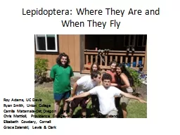
Roy Adams UC Davis Ryan Smith Union College Camila MatamalaOstOregon State Chris Mattioli Providence College in Providence Rhode Island Elizabeth Cowdery Cornell Grace Zalenski ID: 549117
Download Presentation The PPT/PDF document "Lepidoptera: Where They Are and When The..." is the property of its rightful owner. Permission is granted to download and print the materials on this web site for personal, non-commercial use only, and to display it on your personal computer provided you do not modify the materials and that you retain all copyright notices contained in the materials. By downloading content from our website, you accept the terms of this agreement.
Slide1
Lepidoptera: Where They Are and When They Fly
Roy Adams, UC Davis
Ryan Smith, Union College
Camila
Matamala-Ost,Oregon
State
Chris
Mattioli
, Providence College in Providence Rhode Island
Elizabeth
Cowdery
, Cornell
Grace
Zalenski
, Lewis & ClarkSlide2
Lepidoptera
Lepidoptera is second largest class in
Insecta
Approximately 600 species of moths occur in the H.J. Andrews Experimental Forest
Relatively little is knownSlide3
Prey
Defoliators
Pollinators
Decomposers
Diverse Ecological
Roles
Egg
Caterpillar
Pupa
Moth
Ecosystem Functions
Stages of lifecycleSlide4
Pollination
Rodents
Reptiles
Bats
Birds
Spiders
Beetles
True bugs
Nematodes
570 vascular plant species
Ecosystem connections
PreySlide5
Assessing Environmental Impacts
Temperature Caterpillar growth rate affected by temperature
Caterpillar must reach certain critical size to enter
pupal
stage
Majority of moths in Pacific northwest overwinter as egg or in cocoonMany species won’t emerge unless undergo period of cold (dipause)Plant Nutrition
Sensitive to nitrogen and water content
High water content enhances growth
Theoretically, moth abundance and/or emergence could be linked to changes in nitrogen and water content of plants.
Source of food, impacted by abundance of food source, sensitive to changes in temperature and nutritional quality of plants .Slide6
Moth Data and Sampling Slide7
Moth Sampling
Universal Black light traps
22w circular bulbs, 12v batteries
Set 1 – 2 hours before sunset
Moths attracted to light and stunned by insecticide and acrylic veins
Intervals of 1+ weeks
Biased towards
phototatic
night flying moths (majority)
Data not used this summer, will be used in island biogeography studySlide8
Moth IdentificationSlide9
Moth Data Used in Modeling
Sampled with same method by Jeffrey Miller 2004-2008Emergence uses data from 20 sites trapped 30+ timesMoth Distribution includes data from biological inventory survey
Almost 40% sites trapped only once
More than half trapped either once or twice
Feralia
deceptivaSlide10
Vegetation Sampling
Purpose: Test hypothesis that moths are distributed near host plants by contributing to a database of vegetation data at moth sampling sites32 sites
100 meters in 4 directions
All vascular plant species except fern allies (except horsetails)
To learn more about host plants
Polystichum
munitumSlide11
Phenology and Climate Change
“As difficult as it is to predict precisely how the planet will warm over the next century or so, it is even harder to refine predictions of how those changes will affect specific species.”1What are the drivers of moth emergence?
Moths are
poikilothermic
How will climate change influence moth emergence?“Due to human induced climate change over the last decade, phenology has become one of the leading indicators of species’ response to environmental change”2Will this have an effect on other animals?
1:
Barringer
, Felicity. “Trout Fishing in a Climate Changed America.”
New York Times Green
Blog
16/7/2011. 16/7/2011.2: Roy, DB & Sparks, TH. “Phenology of British butterflies and climate
change.” Global Change Biology (2000). 6, 407-416.Slide12
Emergence Objectives
Improve on the previous modelCreate a model that can predict on which day moths will emergeUse degree days instead of Julian days: GDD for plantsSlide13
Model Counts with Julian Days as the interval
Degree-Day Curve Model
Model Showing Counts with Degree Days as intervalSlide14
Degree Days
Took max temp. data from HJ AndrewsAssigned trap sites to Met. and Ref. StandsInterpolated missing dataDiscuss procedure for calculationsSlide15
Thermal Climate of the H.J. Andrews
Experimental
Forest
PRISM estimated mean monthly maximum and minimum temperature maps showing topographic effects of radiation and sky view factors. Provided by Jonathan W.
Smith and EISI 2010Slide16
Formula:=IF(‘VANMET’!B4>0,’VANMET’!B4,0)+'VANMET DEGREE DAYS'!B2Slide17
The Model
Uses abundance data from trapping Estimates parameters of emergence and abundance curves from trap countsOptimizes parameter estimates to create emergence and abundance curvesSlide18
P(j,k)
We assume we catch all moths flying at trap timeP(j,k) is the probability that a moth emerges in interval j and has a natural death time in interval kMeasures abundanceSlide19
Variables
In original model, P(j,k) found by numerically integrating the joint density Q(j,k) and q
j
successively computed
Likelihood function uses
qj to optimize parameter estimates
Emergence time:
Lifespan:Slide20
Obtaining our parameters
= Pr(moth caught by trap)
m
= # moths flying qj = Pr(moth trapped at tj
)
Assume
(a constant) Slide21
Multinomial distributionSlide22
Convergence in distribution
. . .
Where the
F
i
’s
are Poisson random variables
As and , we assume (expected value of moths caught) approaches some constantSlide23
Distribution, cont.
m and alpha are unknownIf m is large and alpha small enough, the likelihood will be very close to PoissonThe model uses the multinomial distribution :Slide24
Incorporating degree days
Degree day values:Each moth has emergence threshold, DNow defineSlide25
Changes
Compute P(j,k) differently because Te is discrete
Single set of parameters for each species, rather than separate for each trap and year
AIC: measure of fitSlide26Slide27Slide28Slide29
3G
Days Since May 1
st
3G
Degree DaysSlide30Slide31
5O
Days Since May 1st5ODegree DaysSlide32Slide33
Future Work
Degree DaysRevisit interpolation methodsExperiment with different degree thresholds and starting datesModelMultinomial v. PoissonMultiple traps for one yearTake new data into account:
Vegetation surveys
Elevation, Aspect, Watershed, HabitatSlide34
Species Distribution Model Applications
Combine numerical observations and relevant variables (often environmental and spatial) to predict species distribution in space and/or timeWhy do this?
Ecological insight, further research topics
Land use management and conservation planningSlide35
SDM’s and Machine Learning
Supervised machine learningUse training data: {(x1,y1), (x2
,y
2
),…,(
xn,yn)} to arrive at a function f(xi) ≈ yi.
Split data into training, test, and validation sets.
Assume that if a moth exists at each site we’ve trapped it at least once at that site.Slide36
SDM’s and Machine Learning
Training set: half of the original data set used in initially learning and fitting the function.Certain algorithms require their parameters to be tuned for optimum performance. This is accomplished by testing the model against a validation set – a subset of the training set.Test set: half of the original data set separate from the training set.After parameter tuning, the function’s accuracy can be evaluated by running it on a test set.Slide37
Quantifying Accuracy
The area under the receiver operating characteristic curve (AUC) is used as our measure of accuracy for the distribution maps.It is the probability that a randomly selected positive instance (moth presence) is ranked higher than a randomly selected negative instance.AUC = 0.5 indicates a random guess.Slide38
Learning Algorithms
AlgorithmsRandom ForestLogistic RegressionSupport Vector MachinesGeneralized Boosted Regression Models
Corresponding R package
randomForest
glmnet
e1071gbmSlide39
Random Forest
Ensemble methodGrows decision trees by combining “bagging” with the random selection of features.A decision tree is a model of decisions and their outcomes. Internal nodes represent points where a decision is made, and the leaves represent the outcomes.“Bagging” is the process of randomly sampling with replacement from the set of training examples, and constructing a decision tree from the “bag”.
Random forest also randomly selects features for each training example rather using the whole of features.Slide40
Random Forest
Plant #1
Pred
#1
Present
Plant #2
Temp
Absent
Present
False
False
False
Absent
Present
True
True
True
High
Low
Temperature
Plant #1
Plant #2
Predetor #1
Moth
1
High
TRUE
TRUE
TRUE
Present
2
Low
TRUE
TRUE
TRUE
Absent
3
Low
TRUE
FALSE
FALSE
Present
4
High
FALSE
TRUE
TRUE
Present
5
Low
FALSE
FALSE
FALSE
AbsentSlide41
Tuning Random Forest
After creating n bags, and growing n trees new data can be classified by taking a vote of all the trees’ predictions.The number of trees grown can be altered and tuned as can the number of nodes of each tree.Slide42
Logistic Regression
P(y = 1|x) = 1/(1+e-t)Where t is (β
0
+
β
1x1 +…+ βnxn)Attempt to find appropriate β values to weigh the covariates.Slide43
Tuning Logistic Regression
It is oftentimes optimal to restrict the number and size of these β values in regression. There is a combination of penalty terms called the “elastic net” to achieve these restrictions.Penalty term takes the form: λ[((1-α)/2)*|
β
|
2
+ (α*|β|)]The parameters: α and λ are tuned.α controls which term is more important.
λ
controls the weight of the entire expression.Slide44
Support Vector Machines
Non-probabilistic classifier.Attempts to construct an n-dimensional hyperplane to separate two possible classes of data.The most desirable hyperplane is the one with the largest functional margin.Slide45
Tuning Support Vector Machines
Oftentimes data is not linearly separable.Kernel functions map the data unto a space where a hyperplane can be easily constructed.LinearRadialSigmoidPolynomialSlide46
Generalized Boosted Regression Models
Ensemble MethodLoss function: a measure that represents the loss in predictive performance of a model.GBM’s construct an initial regression tree that maximally reduces the loss function.A regression tree is a decision tree whose outputs are real-valued.Slide47
Generalized Boosted Regression Models
To further reduce the loss function, new trees are added.At the second step, a regression tree is fitted using the residuals (variations in response) of the first tree.The model now updates to contain two terms, and residuals are taken from the two-term model. The process continues in this stage-wise fashion until a specified parameter – n.trees.
Fitted values update with each new tree addition.Slide48
Tuning GBM
Like the other learning algorithms, GBM also has parameters to be tuned. The number of trees to be constructed and added.The number of nodes in each tree (interaction depth).Slide49
Algorithm Performance
Logistic RegressionRandom Forest
gbm
SVM
Avg
AUC = .605
Avg
AUC = .505
Avg
AUC = .607
Avg
AUC = .606Slide50
Acknowledgements
NSFOSUOSU Arthropod MuseumMatt CoxSteve HighlandTom DietterichDan Sheldon
Olivia
Poblacion
Julia Jones
Desiree TullosJorge RamirezJohn & EmilyVeraJeff Miller/Paul C. Hammond