/
I.1  Diffraction Stack Modeling I.1  Diffraction Stack Modeling

I.1 Diffraction Stack Modeling - PowerPoint Presentation

lily
lily . @lily
Follow
342 views
Uploaded On 2021-01-28

I.1 Diffraction Stack Modeling - PPT Presentation

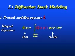
1 Forward modeling operator L d x x x mx dx ò Model Space G model data Integral Equation 2way time Forward Modeling 2way time Forward Modeling Sum of Weighted Hyperbolas ID: 830460

time modeling model data modeling time data model ixtrace matlab diffraction stack cos reflectivity function green

Share:

Link:

Embed:

Download Presentation from below link

Download The PPT/PDF document "I.1 Diffraction Stack Modeling" is the property of its rightful owner. Permission is granted to download and print the materials on this web site for personal, non-commercial use only, and to display it on your personal computer provided you do not modify the materials and that you retain all copyright notices contained in the materials. By downloading content from our website, you accept the terms of this agreement.


Presentation Transcript

Slide1

I.1 Diffraction Stack Modeling

1. Forward modeling operator L

d

(x) =

(x |x’)

m(x’) dx’

ò

Model

Space

G

model

data

Integral

Equation:

Slide2

2-way time

Forward Modeling

Slide3

2-way time

Forward Modeling: Sum of Weighted Hyperbolas

Slide4

G(x|

x’

) =

x

x’

e

iw|x-

x’

|/c

Phase

|x-

x’

|

Geom.

Spread

GREEN’s FUNCTION

|x-

x’

|

Slide5

G(x|

x’

) =

x

x’

e

iw|x-

x’

|/c

Phase

|x-

x’

|

Geom.

Spread

ASYMPTOTIC GREEN’s FUNCTION

A(x

,x’

)

x

x’

+ O( )

-1

x

x’

Slide6

ASYMPTOTIC GREEN’s FUNCTION

G(x|

x’

) =

A(x

,x’

)

x

x’

i

e

x’

x’

R(x’)

reflectivity

Slide7

Diffraction Stack Modeling = ZO Modeling

1-way time

Slide8

Diffraction Stack Modeling = ZO Modeling

2-way time

Dipping Reflector

Slide9

Diffraction Stack Modeling = ZO ModelingIf c for DS is ½ that for ZO Modeling

1-way time

Slide10

ASYMPTOTIC GREEN’s FUNCTION

d(x) =

A(x,x’

)

x

x’

i

e

x’

R(x’)

reflectivity

Fourier Transform:

x

x’

i

e

 (t- )

x

x’

F

~

 (t- )

x

x’

~

d(x)

F

x’

R(x’)

A(x

,x’

)

Slide11

QUICK REVIEW FOURIER TRANSFORM

x

x’

i

e

 (t- )

x

x’

d

( - t)

+

Cos( 2 t )

+

Cos( 4 t )

+

Cos( 3 t )

Cos( t )

t

cancellation

cancellation

constructive

reinforcement @ t=0

 (t)

Slide12

Forward Modeling Operator

 (t- )

x

x’

d(x,t) =

x’

R(x’)

A(x

,x’

)

Sum over reflectivity

Spray energy along

hyperbolas

time

 (t-

)

x

x’

Slide13

Forward Modeling Operator

 (t- )

x

x’

d(x,t) =

x’

R(x’)

A(x

,x’

)

time

REINFORCE

CANCELLATION

W

Slide14

SUMMARY

W (t- )

x

x’

d(x,t) =

x’

Exploding Reflector Modeling = Diffraction Stack Modeling

Single scattering approximation (i.e., Born)

A

(x

,x’

)

R(x’)

reflectivity

Geom. spreading

Source wavelet

Data

variables

Sum over

reflectors

2. High Frequency Approximation (i.e c(x) variations > 3*

 )

3. Approximates Kinematics of ZO Sections, but not Dynamics

d

(x)

= (

x |x’)

m(x’)

dx’

ò

Model

Space

G

model

data

Integral

Equation:

Slide15

MATLAB Exercise: Forward Modeling

W (t- )

x

x’

d(x,t|

x’,0

) =

x’

R(x’)

1. To account for the source wavelet W(t), we

convolve data with W(t)

(recall

 (t-

 )*W(t)= W() )

so that modeling equation becomes (neglect A)

A). Execute MATLAB program forw.m to generate

synthetic data for a point scatterer and a 30 Hz wavelet.

B). Execute MATLAB program forwl.m to generate

synthetic data for a dipping layer model

C). Execute MATLAB program forw.m to generate

synthetic data for a syncline model. Note diffractions

and multiple arrivals. Adjust for new models. Why the

second time derivative?

Slide16

MATLAB Exercise: Forward Modeling

W (t- )

x

x’

d(x,t) =

x’

R(x’)

for ixtrace=1:ntrace;

for ixs=istart:iend;

for izs=1:nz;

r = sqrt((ixtrace*dx-ixs*dx)^2+(izs*dx)^2);

time = 1 + round( r/c/dt );

data(ixtrace,time) = migi(ixs,izs)/r + data(ixtrace,time);

end;

end;

data1(ixtrace,:)=conv2(data(ixtrace,:),rick);end;

* Src Wave

Traveltime

R(x’)

{

Loop over traces

Loop over x in model

Loop over z in model