PDF-Carl von Ossietzky Univers ity Oldenburg Faculty V In

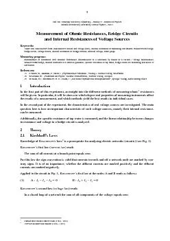
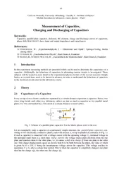
Experimentalphysik 2 Elektrizitt und Optik Springer Verlag Berlin among others 2 TCKER H Taschenbuch der Physik Harri Deutsch Frankfurt 3 ORIES R CHMIDT ALTER H Taschenbuch der Elektrotechnik Harri Deutsch Frankfurt Introduction In this experim. roduction Regional Program ity, possibly infecting the entire store of product).Wash water qualitywater regularly (once per day minimum).levels to maintain 150 ppm to 500 ppm.Provide final rinse if us 79 Named after EORG IMON (1789 1854)USTAV OBERT IRCHHOFF(1824 1887) 80 For this law the sign convention is validthatcurrents towards and off a network node are marked by contrary signs. It is of no im Carl Barks was keenly fascinated with the art of drawing all of his long life. He started as a toddler drawing with small pieces of coal on the walls of his childhood home, and when he reached manhood his skills had been thoroughly developed, although he had had to work with all sorts of odd jobs to make ends meet. Since he was 18, Barks had been drawing cartoons in his spare time in an effort to sell them to local newspapers, but his work was in no great demand until he, as late as in 1928, was contacted by the adult girlie magazine Calgary . Carl Jung. 1875-1961. Freud’s BFF. Friendship ended over furious argument over the nature of the unconscious. Psychotic breakdown. Supported Nazis. Believed all humans share a vast . collective unconscious. The new face for apple!. Who is Carl Brashear?. Diver for the Navy. broke the racial Barrier. Has a prosthetic . leg. He retired from the navy in 1979 after 30 years in the navy. The first black U.S navy diver. ITY OF ORTLANDUREAU OF RANSPORTATIONRob Burchfield, Director of Transportation System Management Sharon White, Program Specialist Clay Veka, Program Coordinator Gabe Graff, High Crash Corridor Supervi PLS. Corey White, Developer. City . of Raleigh Public Utilities. carl.stearns@raleighnc.gov. corey.white@raleighnc.gov. 919-996-2370. Public Utilities GIS Team. Joel Keller. Michael Mazanek. Layman Ricker. EyeOpener. *.. It was just one of that time's several raunchy, pocket-sized men oriented magazines filled with cartoons featuring voluptuous, long-legged blondes and lecherous men, as well as jokes of the often sexually and racially discriminating kind. Barks started out by selling one cartoon for 2 dollars. Now he had a foot in the cartooning world, and he continued to work for the . Born in Stockholm, Sweden. Claes Oldenburg . and Coosjevan Bruggen, his wife. Claes Oldenburg is a Swedish sculptor, best known for his public art installations typically featuring very large replicas of everyday objects. . By: . David . Kristobak. Background. At the age of 13 Watts suffered from meningitis and high fevers and he was pulled out of school for several months.. During his illness he entertained himself by hunting and skinning rabbits.. Laboratory for Underground Nuclear Astrophysics. Reunion . prospective: . Univers. et . Rayons. . Cosmiques. . Why studying nuclear fusion reaction cross sections?. . - . Stars. are powered by . Designed and Drawn By Carl Hock Sept 2011Page 1 of 10 Designed and Drawn By Carl Hock Sept 2011Page 1 of 10 Designed and Drawn By Carl Hock Sept 2011 Designed and Drawn By Carl Hock Sept 2011 1.0 in 1.0 in Designed and Drawn By Carl Hock Sept 2011 1.0 in Designed and Drawn By Carl Hock Sept 2011 Designed and Drawn By Carl Hock Sept 2011 Notches are for light rubber bands used to hold NsdASLA Chspace sywater accommunstate anconstrucOpen spaA retrofit Design This proEnvironof Parks Impervinn Brooklyn New EnglandFirms pe architecdrakedlaapterwt SpecificaDescriptiostem that slctivate