/
EXAMPLE1. Top in at random shuffle. Consider the following method of m EXAMPLE1. Top in at random shuffle. Consider the following method of m

EXAMPLE1. Top in at random shuffle. Consider the following method of m - PDF document

lindy-dunigan
lindy-dunigan . @lindy-dunigan
Follow
430 views
Uploaded On 2015-10-22

EXAMPLE1. Top in at random shuffle. Consider the following method of m - PPT Presentation

a u d d d d c c h b h h FIG I Example of repeated top in at random shuffles of a 4card deck When the original bottom card is at position k from the bottom the waiting time for a new ID: 168658

Share:

Link:

Embed:

Download Presentation from below link

Download Pdf The PPT/PDF document "EXAMPLE1. Top in at random shuffle. Cons..." is the property of its rightful owner. Permission is granted to download and print the materials on this web site for personal, non-commercial use only, and to display it on your personal computer provided you do not modify the materials and that you retain all copyright notices contained in the materials. By downloading content from our website, you accept the terms of this agreement.


Presentation Transcript

EXAMPLE1. Top in at random shuffle. Consider the following method of mixing a deck of cards: the top card is removed and inserted into the deck at a random position. This procedure is repeated a number of times. The following argument should convince the reader that about n log n shuffles suffice to mix up n cards. The argument depends on following the bottom card of the deck. a u d d d d c c h b h h FIG. I. Example of repeated top in at random shuffles of a 4-card deck. When the original bottom card is at position k from the bottom, the waiting time for a new card to be inserted below it is about n/k. Thus the *Research supported by National Science Foundation Grant MCS80-02698. **Research supported by National Science Foundation Grant MCS80-24649. 19861 SHUFFLING CARDS AND STOPPING TIMES 335 analytic proof, and subsequent workers have extended (2.2) to general compact groups-see Grenander (1963), Heyer (1977), Diaconis (1982) for surveys. A version of this result is given here as Theorem 3 of Section 3. Despite this work on abstracting the asymptotic result (2.2), little attention has been paid until recently to the kind of non-asymptotic questions whch are the subject of ths paper. A natural way to measure the difference between two probability distributions Q,, Q, on G is by variation distance There are equivalent definitions where Q(A) = C,,,Q(g), Q(f) = Cf(g)Q(g), and IlfII = maxlf(g)l. Thestring of equalitiesis proved by noting that the maxima occur for A = {g : Q,(g) � Q,(g)) and for f = 1, -1,; Thus, two distributions are close in variation distance if and only if they are uniformly close on all subsets. Plainly 0 llQ, -Q2111. An example may be useful. Suppose, after well-shuffling a deck of n cards, that you happen to see the bottom card, c. Then your distribution Q on S,, is uniform on the set of permutations m for whch m(c) = n, and llQ -UII = 1-l/n. This shows the variation distance can be very "unforgiving" of small deviations from uniformity. Given a distribution Q on a group G, (2.2) says def  (2.4) d,(k) = 1lek*-UII+ 0 ask+ co. Where Q models a random shuffle, d(k) measures how close k repeated shuffles get the deck to being perfectly (uniformly) shuffled. One might suppose d(k) decreases smoothly from (near) 1 to 0; and it is not hard to show d(k) is decreasing. However, THEOREM 1. For the "top in at random" shuffle, Example 1, (a) d(n log n + cn) ep'; all c &#x 000; 0, n &#x 000; 2. (b) d(n1ogn-c,n)+lasn+ w; allc,,+ w. Ths gives a sharp sense to the assertion that n log n shuffles are enough. Ths is a particular case of a general cut-off phenomenon, which occurs in all shuffling models we have been able to analyze; there is a critical number k, of shuffles such that d(k, + o(k,)) -0 but d(k, -o(k,)) = 1. (See Fig. 2.) 19861 SHUFFLING CARDS AND STOPPING TIMES 337 We conclude this section by using Lemma 1 and elementary probability concepts to prove Theorem 1.Here is one elementary result we shall use in several examples. LEMMA 2. Sample uniformly with replacement from an urn with n balls. Let V be the number of draws required until each ball has been drawn at least once. Then Proof. Let m = n log n + cn. For each ball b let A, be the event "ball b not drawn in the first m draws". Then REMARK.This is the famous "coupon-collector's problem", discussed in Feller (1968). The asymptotics are P(V � n log n + cn) + 1-e~p(-e-~)as n + oo, c fixed. So for c not small the bound in Lemma 2 is close to sharp. Proof of Theorem 1. Recall we have argued that T, the first time that the original bottom card has come to the top and been inserted into the deck, is a strong uniform time for this shuffling scheme. We shall prove that T has the same distribution as V in Lemma 2; then assertion (a) is a consequence of Lemmas 1and 2. We can write (2.5) T= TI + (T2 -TI) + ... +(T,-, -T,-2) + (T-T,-,), where q. is the time until the ith card is placed under the original bottom card. When exactly i cards are under the original bottom card b, the chance that the current top card is inserted below i+1 b is -,and hence the random variable q+,-has geometric distribution n  The random variable V in Lemma 2 can be written as (2.7) v= (v-K-,) + (v,-l -K-,) + ... +(v2 -vl) + vl, where is the number of draws required until i distinct balls have been drawn at least once. After i distinct balls have been drawn, the chance that a draw produces a not-previously-drawn n-i ball is -. So v -v-, has distribution n P(y -v-, =j) = - n-i 1 n ) -l j-1 ; �jl. n I Comparing with (2.6), we see that corresponding terms (T+l -?I) and (K -, -K -,-,) have the same distribution; since the summands within each of (2.5) and (2.7) are independent, it follows that the sums T and V have the same distribution, as required. To prove (b), fix j and let A, be the set of configurations of the deck such that the bottom j original cards remain in their original relative order. Plainly U(A,) = l/j! Let k = k(n) be of the form n log n -c,n, c, + oo. We shall show (2.8) Q~*(A,) + 1 asn + oo; jfixed. Then d(k) 2 max {ek*(A,) -U(A,)) + 1as n + oo, establishing part (b). j To prove (2.8), observe ek*(A,) 2 P(T -?;-,� k). For T -I;-, is distributed as the 19861 SHUFFLING CARDS AND STOPPING TIMES 339 This stopping time is clearly a strong uniform time; given that T = 12, all 5 final positions in Z, are equally likely. Such sets of k-tuples can be chosen for any odd n. It turns out that to get the correct rate of convergence, k should be chosen as a large multiple of n2. Here are some details. For fixed integers n and k, with n odd, let B, be the set of binary k-tuples with j pluses (mod M). Let j* be the index corresponding to the smallest IB,, 1. Partition the set of binary k-tuples into n groups of size IB,*l, the jth group being chosen arbitrarily from B,. The random walk generates a sequence of symbols. Consider these in disjoint blocks of length k. Define T as the first time a block equals one of the chosen group. This clearly yields a strong uniform time. The following lemma gives an explicit upper bound for d(k). LEMMA3. Let T be as defined above. For n 2 3 and k 2 n2, P(T � k) g 6e-0~1"~ with a = 4.rr2/3. Proof. The number of elements in B, is this being a classical identity due to C. Ramus (see Knuth (1973, p. 70)). The chance of a given block falling in the chosen group equals Now x Straightforward calculus using quadratic approximations to cosine such as cos x 1--,3 epX2I3for 0 6 x ~/2leads to the stated result. Further details may be found in Chung, Diaconis, and Graham (1986). REMARK.There is a lower bound for d(k) of the form ae-pk/"' for positive a and fi, so somewhat more than n2 steps really are required. One way to prove this is to use the central limit theorem; this implies that after k steps the walk has moved a net distance of order k1/2.Hence we need k of order n2 at least in order that the distribution after k steps is close to uniform. Further details are in Chung, Diaconis and Graham (1986). There is a sense in which the cutoff phenomenon does not occur for tks example. It is possible to show there is a continuous function d*(t), with d*(t) 4 0 as t -co, such that for simple random walk on Z,,, mkmld(k) -d*(k/n2)l 4 0 as n -m. Indeed, as n 4 co, a rescaled version of the random walk tends to Brownian motion on the circle. The function d*(t) is the variation distance to uniformity for Brownian motion at time t. EXAMPLE3. A boundfor generalproblems. Let G be a finite group and Q a probability on G. The following result shows that Q*k converges to the uniform distribution geometrically fast provided Q is not concentrated on a subgroup or a translate of a subgroup. To see the need for this condition, consider Example 2 above (simple random walk on Z,). If n is even, then the 19861 SHUFFLING CARDS AND STOPPING TIMES 341 involves a novel construction of an almost uniform time. For simplicity, we take n = 2' -1 (a common choice in the application). THEOREM4. Let Q, be the probability distribution of X, defined by (3.4) with n = 2' -1. Let d(k) = IlQ, -Ull. Then 1 d(cllogl) +O ash a,�fort - log 3 ' Proof. Observe first that if 6, takes values f1with probability 1/2, then is very close to uniformly distributed mod 2' -1. Indeed, Thus The argument proceeds by finding a stopping time T such that the process stopped at time T has distribution at least as close to uniform as U*. An appropriate modification of the upper bound lemma will complete the proof. We isolate the steps as a sequence of lemmas. The first and second lemmas are elementary with proofs omitted. LEMMA4. Let X,, X,, . . . be a process with ualues in a finite group G. Write Q, for the probability distribution of X,. Let T be a stopping time with the property that for some E � 0, 1lQk(.lT =j) -UII 6 E; allj ,k. Then IIQk -UllG E + P(T � k). LEMMA5. Let Q, and Q2 be probability distributions on a finite group G. Then llQTQ2 -UII llQi -ull. To state the third lemma, an appropriate stopping time T must be defined. Using the defining recurrence X, = 2Xk-, + bk(mod n), (3.6) X, = 2,-'b1 + 2,-,b2 + ... +b,(mod n). Since n = 2' -1, 2' = l(mod n). Group the terms on the right side of (3.6) by distinct powers of 2: with A, = b, + b,,, + b,,,, ...,A, = b, + b,,, + ...,etc. Define T as the first time each of the sums A,, A,, . . . ,A, contains at least one non-zero summand. LEMMA6. The probability distribution of X, given T =j k is the convolution of U* defined above with an independent random variable. 19861 SHUFFLING CARDS AND TIMES 343 is "a permutation with 1or 2 rising sequences". Suppose c cards are initially cut off the top. Then there are ( a) possible riffle shuffles (1 of which is the identity). To see why, label each of the c cards cut with "0"and the others with "1". After the shuffle, the labels form a binary n-tuple with c "0"s: there are (a) such n-tuples and each corresponds to a unique riffle shuffle. Finally, the total number of possible riffle shuffles is Some stage magicians can perform "perfect" shuffles, but for most of us the result of a shuffle is somewhat random. The actual distribution of one shuffle (that is, the set of probabilities of each of the 2" -n possible riffle shuffles) will depend on the skill of the individual shuffler. The following model for random riffle shuffle, suggested by Gilbert and Shannon (1955) and Reeds (1981), is mathematically tractable and qualitatively similar to shuffles done by amateur card players. 1st description. Begin by choosing an integer c from 0,1,. . .,n according to the binomial 1 distribution P{C = c) = -(a). Then, c cards are cut off and held in the left hand, and n -c2" cards are held in the right hand. The cards are dropped from a given hand with probability proportional to packet size. Thus, the chance that a card is first dropped from the left hand packet is c/n. If this happens, the chance that the next card is dropped from the left packet is (c -l)/(n -1). There are two other descriptions of this shuffling mechanism that are useful. 2nd description. Cut an n card deck according to a binomial distribution. If c cards are cut off, pick one of the ( z)possible shuffles uniformly. 3rd description. This generates T-' with the correct probability. Label the back of each card with the result of an independent, fair coin flip as 0 or 1.Remove all cards labelled 0 and place them on top of the deck, keeping them in the same relative order. LEMMA7. The three descriptionsyield the same probability distribution. Proof. The second and third descriptions are equivalent. Indeed, the binary labelling chooses a binomially distributed number of zeros, and conditional on this choice, all possible placements of the zeros are equally likely. The first and second descriptions are equivalent. Suppose c cards have been cut off. For the first description, a given shuffle is specified by a sequence Dl, D,, . . . ,D,, where each D, can be L or R and c of the D,'s must be L. Under the given model, the chance of all such sequences, determined by multiplying the chance at each stage, is c!(n -c)!/n! !J The argument to follow analyzes the repeated inverse shuffle. This has the same distance to uniform as repeated shuffling because of the following lemma. I LEMMA8. Let G be a finite group, T : G + G one-to-one, and Q a probability on G. Then IlQ -ull = llQT-' -ull, where QT-'(g) = Q(T-'(g)) is the probability induced by T. The results of repeated inverse shuffles of n cards can be recorded by forming a binary matrix with n rows. The first column records the zeros and ones that determine the first shuffle, and so on. The ith row of the matrix is associated to the i th card in the original ordering of the deck, recording in coordinate j the behavior of this card on the jth shuffle. 19861 SHUFFLING CARDS AND STOPPING TIMES 345 REMARK(b). The argument can be refined. Suppose shuffling is stopped slightly before all rows of the matrix are distinct-e.g., stop after 210g n shuffles. Cards associated to identical binary rows correspond to cards in their original relative positions. It is possible to bound how far such permutations are from uniform and get bounds on -UII. Reeds (1981) has used such arguments to show that 9 or fewer shuffles make the variation distance small for 52 cards. REMARK(c). A variety of ad hoc techniques have been used to get lower bounds. One simple method that works well is to simply follow the top card after repeated shuffles. This executes a Markov chain on n states with a simple transition matrix. For n in the range of real deck sizes, n X n matrices can be numerically multiplied and then the variation distance to uniform computed. Reeds (1981) has carried this out for decks of size 52 and shown that -U 11 � .I. Techniques which allow asymptotic verification that k = (3/2)log, n is the right cutoff for large n are described in Aldous (1983a). These analyses, and the results quoted above, suggest that seven riffle shuffles are needed to get close to random. REMARK (d). Other mathematical models for riffle shuffling are suggested in Donner and Uppulini (1970), Epstein (1977), and Thorp (1973). Bore1 and Cheron (1955) and Kosambi and Rao (1958) discuss the problem in a less formal way. Where conclusions are drawn, 6 to 7 shuffles are recommended to randomize 52 cards. REMARK(e). Of course, our ability to shuffle cards depends on practice and agility. The model produces shuffles with single cards being dropped about 1/2 of the time, pairs of cards being dropped about 1/4 of the time, and i cards blocks being dropped about 1/2' of the time. Professional dealers drop single cards 80% of the time, pairs about 18% of the time and hardly ever drop 3 or more cards. Less sophisticated card handlers drop single cards about 60% of the time. Further discussion is in Diaconis (1982) or Epstein (1977). It is not clear if neater shuffling makes for a better randomization mechanism. After all, eight perfect shuffles bring a deck back to order. Diaconis, Kantor, and Graham (1983) contains an extensive discussion of the mathematics of perfect shuffles, giving history and applications to gambling, computer science and group theory. The shuffle analyzed above is the most random among all single shuffles with a given distribution of cut size, being uniform among the possible outcomes. It may therefore serve as a lower bound; any less uniform shuffle might take at least as long to randomize things. Further discussion is in Mellish (1973). REMARK(f). One may ask, "Does it matter?" It seems to many people that if a deck of cards is shuffled 3 or 4 times, it will be quite mixed up for practical purposes with none of the esoteric patterns involved in the above analysis coming in. Magicians and card cheats have long taken advantage of such patterns. Suppose a deck of 52 cards in known order is shuffled 3 times and cut arbitrarily in between these shuffles. Then a card is taken out, noted and replaced in a different position. The noted card can be determined with near certainty! Gardner (1977) describes card tricks based on the inefficiency of too few riffle shuffles. Berger (1973) describes a different appearance of pattern. He compared the distribution of hands at tournament bridge before and after computers were used to randomize the order of the deck. The earlier, hand shuffled, distribution showed noticeable patterns (the suit distributions were too near "even" 4333) that a knowledgeable expert could use. It is worth noting that it is not totally trivial to shuffle cards on a computer. The usual method, described in Knuth (1981), goes as follows. Imagine the n cards in a row. At stage i, pick a random position between i and n and switch the card at the chosen position with the card at position i. Carried out for 1i n -1, this results in a uniform permutation. the early days of computer randomization, we are told that Bridge Clubs randomized by choosing about 60 random transpositions (as opposed to 51 carefully randomized transpositions). As the analysis of 19861 SHUFFLING CARDS AND STOPPING TIMES 347 bounds. Letac (1981) and Takhcs (1982) are readable surveys. Diaconis and Shahshahani (1981, 1984) present further examples. Robbins and Bolker (1981) use other techniques. Despite this range of available techniques, there are some shuffling methods for which we do not have good results on how many shuffles are needed; for example: (i) Riffle shuffles where there is a tendency for successive cards to be dropped from opposite hands. (ii) Overhand shuffle, The deck is divided into K blocks in some random way, and the order of the blocks is reversed. (iii) Semi-random transposition. At the k th shuffle, transpose the k th card (counting modulo n) with a uniform random card. From a theoretical viewpoint, there are interesting questions concerning the cut-off phenomenon. This occurs in all the examples we can explicitly calculate, but we know no general result which says that the phenomenon must happen for all "reasonable" shuffling methods. Acknowledgment. We thank Brad Efron, Leo Flatto, and Larry Shepp for help with Example 1, and Jim Reeds for help with Section 4. References D. Aldous, Markov chains with almost exponential hitting times, Stochastic Proc. Appl., 13 (1982) 305-310. , Random walks on finite groups and rapidly mixing Markov chains, Skminaire de Probabilitks, XVII (1983a) 243-297. , Minimization algorithms and random walk on the d-cube, Ann. Probab., 11 (1983b) 403-413. D. J. Aldous and P. Diaconis, Uniform stopping times for random walks on groups, 1985. In preparation. K. B. Athreya and P. Ney, A new approach to the limit theory of recurrent Markov chains, Trans. Amer. Math. SOC., 1977. K. B. Athreya, D. McDonald, and P. Ney, Limit theorems for semi-Markov processes and renewal theory for Markov chains, Ann. Probab., 6 (1978) 788-797. P. Berger, On the distribution of hand patterns in bridge: man-dealt versus computer-dealt, Canad. J. Statist., 1 (1973) 261-266. E. Bore1 and A. Cheron, Thkorie Mathkmatique du Bridge, 2nd ed.. Gauthier Villars, Paris, 1955. A. Broder, unpublished, Stanford University, 1985. F. K. Chung, P. Diaconis, and R. L. Graham, Random walks arising from random number generation, Technical Report #212, Stanford University, 1983 (to appear. Ann. Probab.). P. Diaconis (1982), the use of group representations in probability and statistics. Typed Lecture Notes, Department of Statistics, Harvard University. To appear, Institute of Mathematical Statistics. P. Diaconis, W. Kantor, and R. L. Graham, The mathematics of perfect shuffles, Advances in Applied Math., 4 (1983) 175-196. P. Diaconis and M. Shahshahani, Generating a random permutation with random transpositions. Z. Wahrsch. Venv. Gebiete, 57 (1981) 159-179. ,Factoring probabilities on compact groups, Technical Report #178, Stanford University (also TR#PH- 9, Haward Univ.) 1986 (to appear, Proc. Amer. Math. Soc.). , Products of random matrices and random walks on groups. To appear, Proc. Conference on Random Matrices (J. Cohen, H. Kesten, C. Newman, eds.), Amer. Math. Providence, RI, l9,84. J. R. Donner and V. R. R. Uppulini, A Markov chain structure for riffle shuffling, SIAM J. Appl. Math., 18 (1970) 191-209. R. Epstein, The Theory of Gambling and Statistical Logic, Revised ed., Academic Press, New York. 1977. W. Feller, An Introduction to Probability and Its Applications, Vol. I, 3rd ed., Wiley, New York, 1968. L. Flatto, A. Odlyzko, and D. Wales, Random shuffles and group representations. Ann. Probab., 13 (1985) 181-193. M. Gardner, Mathematical Magic Show, Knopf, New York, 1977. E. W. Gilbert, Theory of Shuffling, Bell Laboratories Technical Memorandum. Murray Hill, NJ, 1955. U. Grenander, Probability on Algebraic Structures, Wiley, New York, 1963. D. Griffeath, A maximal coupling for Markov chains, Z. Wahrsch. Venv. Gebiete, 31 (1975) 95-106. ,Coupling methods for Markov processes, in Studies in Probability and Ergodic Theory, Adv, in Math., Supplementary Studies Vol. 2 (J. C. Rota ed.), (1978) 1-43.