/
GeoTASO: An airborne GeoTASO: An airborne

GeoTASO: An airborne - PowerPoint Presentation

lindy-dunigan
lindy-dunigan . @lindy-dunigan
Follow
380 views
Uploaded On 2017-10-29

GeoTASO: An airborne - PPT Presentation

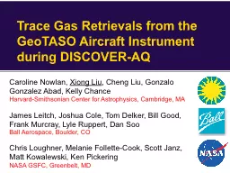
testbed for TEMPO and GEMS trace gas retrievals Caroline Nowlan Xiong Liu Gonzalo Gonzalez Abad Kelly Chance Peter Zoogman HarvardSmithsonian Center for Astrophysics Cambridge MA James Leitch Joshua Cole Tom ID: 600735

data geotaso resolution level geotaso data level resolution no2 discover retrievals colorado spatial stray light fwhm pixels slit texas

Share:

Link:

Embed:

Download Presentation from below link

Download Presentation The PPT/PDF document "GeoTASO: An airborne" is the property of its rightful owner. Permission is granted to download and print the materials on this web site for personal, non-commercial use only, and to display it on your personal computer provided you do not modify the materials and that you retain all copyright notices contained in the materials. By downloading content from our website, you accept the terms of this agreement.


Presentation Transcript

Slide1

GeoTASO: An airborne testbed for TEMPO and GEMS trace gas retrievals

Caroline Nowlan, Xiong Liu, Gonzalo Gonzalez Abad, Kelly Chance, Peter ZoogmanHarvard-Smithsonian Center for Astrophysics, Cambridge, MAJames Leitch, Joshua Cole, Tom Delker, Bill Good, Frank Murcray, Lyle Ruppert, Dan Soo Ball Aerospace, Boulder, COChris Loughner, Melanie Follette-Cook, Scott Janz, Matt Kowalewski, Ken PickeringNASA GSFC, Greenbelt, MDJay al-SaadiNASA LaRC, Hampton, VATEMPO Science Team Meeting, 1-2 June 2016Slide2

How GeoTASO Informs TEMPO

Sensor-algorithm interactions and key parametersIdentifies sensor artifacts that influence retrieval accuracyHighlights tests and measurements needed for good retrievalsCan conversely show where sensor performance and testing can be relaxedAlgorithm preparation/tuning for TEMPOOffers direct test of algorithm performance vs. SNR and spectral passband/samplingTests surface reflectance effects on retrievalsDemonstrate combined UV/Visible ozone retrievalHigh spatial resolution checks for any smaller scale effects on space-based retrievals(Jim Leitch, GeoTASO IIP Final Review 2014)

Satellite analogue for preparatory field campaigns

Future validation instrumentSlide3

GeoTASO InstrumentSlide4

GeoTASO InstrumentGeostationary Trace gas and Aerosol Sensor OptimizationMeasures with two 2D CCD detector

arrays (UV and VIS)GeoTASOTEMPOWavelength range290 – 400 nm (UV)415 – 695 nm (VIS)290 – 490 nm (UV)540 – 740 nm (VIS)Nominal spectral sampling3.1 pixels/FWHM2.9 pixels/FWHMNominal spectral resolution0.43 nm (UV)0.88 nm (VIS)0.57 nmNative spatial resolution

9

m x 50 m

2.1 km

x 4.4 km

Reference

spectrum

Zenith or clean

nadir

Solar diffuserSlide5

GeoTASO Campaigns

CampaignLocationDatesTest flightsVirginia/MarylandJuly 2013DISCOVER-AQTexasSeptember 2013DISCOVER-AQColoradoJuly-August 2014Ocean colorNOAA ship, off VirginiaJuly 2015KORUS-AQKoreaMay-June 2016

NO2 retrievals from DISCOVER-AQ Texas 2013 available online on NASA data archive

Nowlan et al., AMTD, 2015

L1B data for DISCOVER-AQ Colorado is available from NASA ftp as of May 2016 (contact Jay al-

Saadi

)Slide6

GeoTASO SpectrometerSlide7

GeoTASO Observations

Native resolution is ~9 m x 50 m with SNR=65 (NO2) and SNR=110 (HCHO)Co-add to reduce noise For NO2, we provide data at 250 m x 250 mSlide8

Trace Gas RetrievalsSlide9

NO2 over Downtown Houston13 September 2013

VerticalColumnSlide10

NO2 over Downtown Houston13 September 2013Slide11

NO2 over Denver, Raster Scans2 August 2014

8:00 – 11:30 AM Local time2:00 – 4:00 pm local timeSlantColumnSlide12

Colorado FormaldehydeSlide13

Denver HCHOSlide14

O3 Profiles

PreliminaryUV-only retrievalUse UV and Visible channels to test O3 profile retrievalsSome challenges:Absolute radiometric calibrations need to be very accurateDevelopment of a good reference spectrumSlide15

GeoTASO SO2

Photo by J.B. ForbesGeoTASO measured coincident slant columns of NO2 and SO2 downwind from Labadie Power Station, Missouri’s largest coal-burning power plant, on transit from Colorado to Virginia (08/13/2014)Slide16

Calibration, Characterization and Level 2 Data QualitySlide17

Characterization using Flight Data:BackgroundSlit function shape parameters and wavelength dispersion are fit before trace gas retrieval using a high-resolution solar reference spectrum (i.e., Chance and

Kurucz, 2010)See Liu et al., 2005 (GOME), Liu et al., 2010 (OMI), Cai et al., 2012 (GOME-2)For aircraft data, need to fit “pseudo-absorbers” (O3 etc.) at the same time as we do not have an exo-atmospheric spectrumSlide18

Characterization using Flight Data:Slit Function

Slit function shapes and widths are very stable across both dimensions of CCD array (<0.01 nm differences).Slide19

Wavelength

sampling varies across spatial dimensionZenith spectra are collected at center of array using optical fiberFitting a wavelength shift relative to zenith reference in retrieval works fine for NO2HCHO is more sensitive to calibration errors, and cross-track dependent clean nadir reference works bestCharacterization using Flight Data:Wavelength RegistrationSlide20

Level 0 to Level 1B ProcessingRemove dark currentCorrect for:

OffsetCrosstalkSmearOut-of-band straylightOut-of-field straylightConvert to scene radiance using radiometric calibration data GeolocationSlide21

Level 0 to Level 1B Processing:Noise introduced by calibrationsStray light corrections have spectral noise

These can be smoothed, or else will introduce noise that increases fitting residualsA persistent pattern shows up in all spectra in L0L1B version with stray light smoothing turned off.Slide22

Regions of high RMS correlate with bright red-brown fields (bare soil?)

Likely from incorrect out-of-band stray light correction Luckily, the Colorado campaign had few of these observations.RMSRGB ImageLevel 0 to Level 1B Processing:Red field effect in NO2 retrievalsSlide23

Level 0 to Level 1B Processing: Along-Track StripingSaturated pixels at edge of cross-track view can bleed into out-of-field detector pixels which are used for stray light corrections

Along-track striping in Level 2 retrievals can appear if stray light is not removed correctlyRaw CCD frameSlide24

Effects of Slit SizeGeoTASO was designed to take replaceable slits of varying sizes

DISCOVER-AQ Texas used four slit sizes on different flights26.0 mm32.5 mm39.0 mm45.5 mmUV sampling (pixels/FWHM)2.52.83.13.5VIS sampling (pixels/FWHM)2.5

2.7

3.1

3.6

UV FWHM (nm)

0.34

0.39

0.43

0.49

VIS FWHM (nm)

0.70

0.75

0.88

1.00

undersampledSlide25

Effects of Slit Size (NO2)

SNR is lower for narrower slitsIntegration time was the same for all flightsCost of low throughput not offset by benefits of higher spectral resolution for two narrowest slitsDISCOVER-AQ Texas NO2 Fitting Uncertainties Slide26

ValidationSlide27

GeoTASO NO2 vs PANDORA NO2 Houston Urban Flights

NO2 at 250 m x 250 m resolution has fitting uncertainty of 2.2e15 molecules/cm2TEMPO will have coarser spatial resolution (2.1x4.4 km2) and higher precisionExpect similar features (correlation increases with range of NO2) but lower slope (lower spatial resolution) and reduced

r (lower spatial and temporal resolution)Slide28

GeoTASO NO2 vs In Situ NO2 Houston Urban Flights

(Following Lamsal et al., 2008)Slide29

Current Status and SummaryL1B dataDISCOVER-AQ Texas available

UV data contaminated by stray lightContact Jim Leitch at Ball Aerospace or Caroline at SAODISCOVER-AQ Colorado available as of May Contact Jay al-SaadiLevel 2 dataDISCOVER-AQ Texas NO2 on data archiveDISCOVER-AQ Colorado non-final results available from SAOSee Nowlan et al. (2015, AMTD)Instrument currently deployed in KORUS-AQBall has transferred instrument to Scott Janz at NASA GSFC