International Journal of Computer Science & Engineering Survey (IJCSES - PDF document

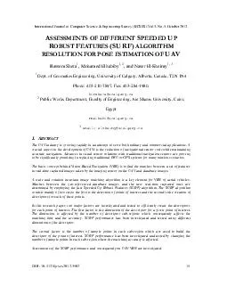
International Journal of Computer Science & Engineering Survey (IJCSES) Vol.3, No.5, October 2012 DOI : 10.5121/ijcses.2012.3502 15  \n \r\n\n\r
 
 \r
 
Bassem Sheta, Mohamed Elhabiby1, 2, and Naser El-Sheimy1, 3 Dept. of Geomatics Engineering, University of Calgary, Alberta, Canada, T2N 1N4 Phone: 403-210-7897, Fax: 403-284-1980, bimsheta@ucalgary.ca Public Works Department, Faculty of Engineering, Ain Shams University, Cairo, Egypt mmelhabi@ucalgary.ca Email: elsheimy@ucalgary.ca1.BSTRACTThe UAV industry is growing rapidly in an attempt to serve both military and commercial applications. A crucial aspect in the development of UAVs is the reduction of navigational sensor costs while maintaining accurate navigation. Advances in visual sensor solutions with traditional navigation sensors are proving to be significantly promising in replacing traditional IMU or GPS systems for many mission scenarios. The basic concept behind Vision Based Navigation (VBN) is to find the matches between a set of features in real-time captured images taken by the imaging sensor on the UAV and database images. A scale and rotation invariant image matching algorithm is a key element for VBN of aerial vehicles. Matches between the geo-referenced database images and the new real-time captured ones are determined by employing the fast Speeded Up Robust Features (SURF) algorithm. The SURF algorithm consists mainly of two steps: the first is the detection of points of interest and the second is the creation of descriptors for each of these points. In this research paper, two major factors are investigated and tested to efficiently create the descriptors for each point of interest. The first factor is the dimension of the descriptor for a given point of interest. The dimension is affected by the number of descriptor sub-regions which consequently affects the matching time and the accuracy. SURF performance has been investigated and tested using different dimensions of the descriptor. The second factor is the number of sample points in each sub-region which are used to build the descriptor of the point of interest. SURF performance has been investigated and tested by changing the number of sample points in each sub-region where the matching accuracy is affected. Assessments of the SURF performance and consequently on UAV VBN are investigated. International Journal of Computer Science & Engineering Survey (IJCSES) Vol.3, No.5, October 2012 16 2.KEYWORDS UAV, Vision Based Navigation, Speeded Up Robust Features (SURF) 3.NTRODUCTIONIn order to address vision-aided navigation problems, two important approaches for navigation should be discussed: non-inertial vision navigation methods and inertially-aided vision navigation. 3.1Non-inertial Vision Navigation Methods An approach was proposed by [1] for estimating an aircraft’s position and orientation using visual measurements for landmarks located on a known topographic map using an extended Kalman filter. In this approach, landmarks, referred to as “tokens”, are detected based on maximizing a uniqueness measure that prevents such tokens from being too close to each other as the terrain around them is linear. The uniqueness measure detects the point of interest in the matching algorithm based on the spatial distance and feature distance between points of interest candidates. Then, those tokens are described based on circular integrals of pixel intensities: ()(cos,sin) iii ePfxryrd p aaa =++Eq. 1 Where P(x,y) is a point in the image [1]. Such descriptors are invariant for translation and rotation. Another approach for estimating aircraft position and velocity from sequential aerial images was proposed by [2, 3]. This method in [3] provides real-time implementation of a vision-based navigation algorithm which accomplishes both accuracy and effectiveness (in other words the cheapness of the sensors used, computational load and complexity).The new algorithm is composed of two sections: relative and absolute position estimation , which are connected to each other through a switching scheme. The relative position estimation section is essentially based on the stereo modelling of two sequential images where the feature point of a current and previous image is utilized for extracting the displacement of the aircraft. This is achieved by applying the Block Matching Algorithm (BMA) and Normalized Correlation Coefficient (NCC) where two levels of Gaussian-based hierarchical matching are used to lower the computational load of the algorithm. Accumulation of the displacement calculation leads to a position measurement for the aircraft. The velocity of the aircraft is then obtained by dividing these displacements by the sampling interval time. However, accumulating these displacement measurements yields errors in navigation parameters estimation subsequently increasing with time as well. The next step involves estimating the absolute position, which corrects the errors arising due to the accumulation of displacement measurements performed through relative position estimation. This is achieved through matching schemes using reference images (if the effective range from the reference position is 400 m and distinct artificial landmarks are available in the scene) and Digital Elevation Model (DEM) (if the effective range is 200m and areas where no artificial landmarks are available). International Journal of Computer Science & Engineering Survey (IJCSES) Vol.3, No.5, October 2012 17 3.2Inertially–aided Vision Navigation Object detection and avoidance for aerial vehicles was addressed in [4, 5]. The proposed approach fused inertial measurements with information that originated from image sequences to calculate range measurements for estimating the object distance. The algorithm consists of the following steps based on two frames taken at times t1 and t2: 1.For the two frames, calculate the navigation state of each image using the inertial data. 2.Extract interest points from each frame. 3.Locate the focus of expansion using the velocity vector from inertial measurements. 4.Project the focus of expansion and interest points in the second frame onto an image plane parallel to the first frame. 5.Match the interest points from the second frame to the interest points from the first frame. 6.Compute the range to each interest point. 7.Create dense range maps using the computed range values to obstacles. Interest points are detected using the Hessian and Laplacian operators as the following: () xyxxyy Igggg =-Eq. 2 Where is the gray level function and xx is the second derivative in the direction [5]. This approach however, was just an initial solution for integrating inertial with vision measurements to help obstacle avoidance. It showed the importance of using inertial measurements to help solve the correspondence problem [6]. Another application that uses the augmentation of inertial measurements with image-based motion estimation was presented in [7]. This approach was proposed for helping NASA missions achieve accurate and safe landings on planetary bodies. The sensors used in this algorithm are INS, laser altimeter, and image sensor. Additionally, the applied image-based motion estimation approach can be categorized as a two-frame feature based motion estimation. The measurements, originating from those sensors, are fused through a modified Kalman filter which estimates the errors in the estimated states for vehicle navigation. The proposed VBN approach is based on locating the correspondence points between a set of features in real-time captured images taken by the imaging sensor on the UAV and database images. These correspondence points between the geo-referenced database images and those captured in real-time are found by employing the fast Speeded Up Robust Features (SURF) algorithm. In this research paper, two major factors are investigated and tested to efficiently create the descriptors for each point of interest. The first factor is the dimension of the descriptor for point of interest. The second is the number of sample points in each sub-region which is used to build the descriptor of the point of interest. 4.ETHODOLOGYThe image matching algorithms play a key role in the VBN. Table 1 summarizes the most important research work done in image matching along with the corresponding techniques used. International Journal of Computer Science & Engineering Survey (IJCSES) Vol.3, No.5, October 2012 18 Table 1 Summary of past work on image matching Reference Matching technique Advantages and Disadvantages [8] Pixel by pixel correlation Computationally, expensive and are scale and rotation variants. [9] Bounded partial correlation Reduced computation. [10] Weighted least square Used in target tracking where the basic error kernel was modified [11] Block matching Reduced computation through parallel computation [12] [13] PCA and wavelets Rotation invariant texture identification [14] Chamfer matching Edge detected images are used instead of pixels [15] Multi-resolution matching Reduced computation through lower resolution [16] Corner matching Used in high resolution images [17] Frequency domain image matching Speed optimization [18] L4 template matching Faster approach in frequency domain matching [19] Shape based matching Descriptors are based on geometric blur point which calculates the cost function [20] [21] Affine image matching Shape features are represented by the Fourier descriptors [22] Multi-scale template matching Linear combination of Haar-like template binary features is used [23] [24] Scale Invariant Feature Transform High accuracy and relatively low computation time, and rotation and scale invariance In this paper, matches between the geo-referenced database images and those captured in real-time are locating by employing the fast SURF algorithm. SURF, sometimes referred to as the Fast-Hessian detector, is essentially based on the Hessian matrix with Laplacian-based detectors such as Difference of Gaussian (DoG) [25]. SURF descriptors describes the gradient information in the point of interest neighbourhood through Haar wavelet responses [26]. The algorithm consists mainly of two steps. The first is the detection of points of interest and the second is the creation of descriptors for each point. The integral image approach is used to improve the performance of the algorithm and computational time prospective. The block diagram for the SURF algorithm is shown in Figure 1. International Journal of Computer Science & Engineering Survey (IJCSES) Vol.3, No.5, October 2012 4.1Interest point detection To achieve fast robust features, the SURF algorithm employs the integral images approach which reduces the computation time. 4.1.1Integral images Occasionally, t his approach is the summed area table image from the summing of pixels’ intensities of the input image I within a rectangular region formed around location x as the following Points of Interests Desription Determine the descriptor size Points of Interest Extraction &#x/Pre; ict;&#xor 1; /C;&#xolum;&#xns 1;ė ;&#x/Col;&#xors ;　&#x/Pre; ict;&#xor 1; /C;&#xolum;&#xns 1;ė ;&#x/Col;&#xors ;　ÅýYÔjZC,&|I_^a2J‡jšÆ9ÇðP¼ÂXka Æ˜6F&#x/Pre; ict;&#xor 1; /C;&#xolum;&#xns 1;ė ;&#x/Col;&#xors ;　&#x/Pre; ict;&#xor 1; /C;&#xolum;&#xns 1;ė ;&#x/Col;&#xors ;　ÅýYÔjZC,&|I_^a2J‡jšÆ9ÇðP¼ÂXka Æ˜6F&#x/Pre; ict;&#xor 1; /C;&#xolum;&#xns 1;ė ;&#x/Col;&#xors ;　&#x/Pre; ict;&#xor 1; /C;&#xolum;&#xns 1;ė ;&#x/Col;&#xors ;　zÍýª½“IÏÕÿÐ__† EI Q q 1117 0 0 1 736.996 4377 cm BI /CS/RGB /W 1117 /H 1 /BPC 8 /F/Fl /DPÏ·âNY&#x/Pre; ict;&#xor 1; /C;&#xolum;&#xns 1;ė ;&#x/Col;&#xors ;　&#x/Pre; ict;&#xor 1; /C;&#xolum;&#xns 1;ė ;&#x/Col;&#xors ;　&#x/Pre; ict;&#xor 1; /C;&#xolum;&#xns 1;ė ;&#x/Col;&#xors ;　&#x/Pre; ict;&#xor 1; /C;&#xolum;&#xns 1;ė ;&#x/Col;&#xors ;　|XžÒ?ò_
ow`‹ EI Q q 1117 0 0 1 736.996 4376 cm BI /CS/RGB /W 1117 /H 1 /BPC 8 /F/Fl /DP|XžÒ?ò_
ow`‹ EI Q q 1117 0 0 1 736.996 4376 cm BI /CS/RGB /W 1117 /H 1 /BPC 8 /F/Fl /DP&#x/Pre; ict;&#xor 1; /C;&#xolum;&#xns 1;ė ;&#x/Col;&#xors ;　&#x/Pre; ict;&#xor 1; /C;&#xolum;&#xns 1;ė ;&#x/Col;&#xors ;　&#x/Pre; ict;&#xor 1; /C;&#xolum;&#xns 1;ė ;&#x/Col;&#xors ;　&#xݕvH;ÌDI;&#x²/n;&#xʈ6¨;&#xºÛ©";&#xˆºC#;&#xÿ‹Ÿ2; ÷ ;&#x«’^‹;&#x`Ä;&#x[d0;&#x/Pre; ict;&#xor 1; /C;&#xolum;&#xns 1;ė ;&#x/Col;&#xors ;　&#x/Pre; ict;&#xor 1; /C;&#xolum;&#xns 1;ė ;&#x/Col;&#xors ;　&#x/Pre; ict;&#xor 1; /C;&#xolum;&#xns 1;ė ;&#x/Col;&#xors ;　“ALàâ:15ò?AkQ“ EI Q q 1117 0 0 1 736.996 4374 cm BI /CS/RGB /W 1117 /H 1 /BPC 8 /F/Fl /DP“ALàâ:15ò?AkQ“ EI Q q 1117 0 0 1 736.996 4374 cm BI /CS/RGB /W 1117 /H 1 /BPC 8 /F/Fl /DP“ALàâ:15ò?AkQ“ EI Q q 1117 0 0 1 736.996 4374 cm BI /CS/RGB /W 1117 /H 1 /BPC 8 /F/Fl /DP&#x/Pre; ict;&#xor 1; /C;&#xolum;&#xns 1;ė ;&#x/Col;&#xors ;　&#x/Pre; ict;&#xor 1; /C;&#xolum;&#xns 1;ė ;&#x/Col;&#xors ;　&#x/Pre; ict;&#xor 1; /C;&#xolum;&#xns 1;ė ;&#x/Col;&#xors ;　 7"Â{úã]QGój§;ñ_bš EI Q q 1117 0 0 1 736.996 4373 cm BI /CS/RGB /W 1117 /H 1 /BPC 8 /F/Fl /DP&#x/Pre; ict;&#xor 1; /C;&#xolum;&#xns 1;ė ;&#x/Col;&#xors ;　&#x/Pre; ict;&#xor 1; /C;&#xolum;&#xns 1;ė ;&#x/Col;&#xors ;　&#x/Pre; ict;&#xor 1; /C;&#xolum;&#xns 1;ė ;&#x/Col;&#xors ;　&#x/Pre; ict;&#xor 1; /C;&#xolum;&#xns 1;ė ;&#x/Col;&#xors ;　&#x/Pre; ict;&#xor 1; /C;&#xolum;&#xns 1;ė ;&#x/Col;&#xors ;　&#x/Pre; ict;&#xor 1; /C;&#xolum;&#xns 1;ė ;&#x/Col;&#xors ;　&#x/Pre; ict;&#xor 1; /C;&#xolum;&#xns 1;ė ;&#x/Col;&#xors ;　&#x/Pre; ict;&#xor 1; /C;&#xolum;&#xns 1;ė ;&#x/Col;&#xors ;　
íHÑJN«:ñÛÿ ?Ád£ EI Q q 1117 0 0 1 736.996 4372 cm BI /CS/RGB /W 1117 /H 1 /BPC 8 /F/Fl /DP
íHÑJN«:ñÛÿ ?Ád£ EI Q q 1117 0 0 1 736.996 4372 cm BI /CS/RGB /W 1117 /H 1 /BPC 8 /F/Fl /DP&#x/Pre; ict;&#xor 1; /C;&#xolum;&#xns 1;ė ;&#x/Col;&#xors ;　&#x/Pre; ict;&#xor 1; /C;&#xolum;&#xns 1;ė ;&#x/Col;&#xors ;　
íHÑJN«:ñÛÿ ?Ád£ EI Q q 1117 0 0 1 736.996 4372 cm BI /CS/RGB /W 1117 /H 1 /BPC 8 /F/Fl /DP
íHÑJN«:ñÛÿ ?Ád£ EI Q q 1117 0 0 1 736.996 4372 cm BI /CS/RGB /W 1117 /H 1 /BPC 8 /F/Fl /DP&#x/Pre; ict;&#xor 1; /C;&#xolum;&#xns 1;ė ;&#x/Col;&#xors ;　&#x/Pre; ict;&#xor 1; /C;&#xolum;&#xns 1;ė ;&#x/Col;&#xors ;　
íHÑJN«:ñÛÿ ?Ád£ EI Q q 1117 0 0 1 736.996 4372 cm BI /CS/RGB /W 1117 /H 1 /BPC 8 /F/Fl /DP&#x/Pre; ict;&#xor 1; /C;&#xolum;&#xns 1;ė ;&#x/Col;&#xors ;　&#x/Pre; ict;&#xor 1; /C;&#xolum;&#xns 1;ė ;&#x/Col;&#xors ;　&#x/Pre; ict;&#xor 1; /C;&#xolum;&#xns 1;ė ;&#x/Col;&#xors ;　L§cÏë+ô™ÛýQ=Ô+¢Ö±Ý%茨¡ŽIËÒáÝ·½
ËHÎ EI Q q 1117 0 0 1 736.996 4367 cm BI /CS/RGB /W 1117 /H 1 /BPC 8 /F/Fl /DP&#x/Pre; ict;&#xor 1; /C;&#xolum;&#xns 1;ė ;&#x/Col;&#xors ;　&#x/Pre; ict;&#xor 1; /C;&#xolum;&#xns 1;ė ;&#x/Col;&#xors ;　&#x/Pre; ict;&#xor 1; /C;&#xolum;&#xns 1;ė ;&#x/Col;&#xors ;　L§cÏë+ô™ÛýQ=Ô+¢Ö±Ý%茨¡ŽIËÒáÝ·½
ËHÎ EI Q q 1117 0 0 1 736.996 4367 cm BI /CS/RGB /W 1117 /H 1 /BPC 8 /F/Fl /DPL§cÏë+ô™ÛýQ=Ô+¢Ö±Ý%茨¡ŽIËÒáÝ·½
ËHÎ EI Q q 1117 0 0 1 736.996 4367 cm BI /CS/RGB /W 1117 /H 1 /BPC 8 /F/Fl /DP&#x/Pre; ict;&#xor 1; /C;&#xolum;&#xns 1;ė ;&#x/Col;&#xors ;　&#x/Pre; ict;&#xor 1; /C;&#xolum;&#xns 1;ė ;&#x/Col;&#xors ;　&#x/Pre; ict;&#xor 1; /C;&#xolum;&#xns 1;ė ;&#x/Col;&#xors ;　&#x/Pre; ict;&#xor 1; /C;&#xolum;&#xns 1;ė ;&#x/Col;&#xors ;　&#x/Pre; ict;&#xor 1; /C;&#xolum;&#xns 1;ė ;&#x/Col;&#xors ;　™2—áÊìI‹y¥ÂS‘ aGÑ:|~õ½‰™2—áÊìI‹y¥ÂS‘ aGÑ:|~õ½‰™2—áÊìI‹y¥ÂS‘ aGÑ:|~õ½‰&#x/Pre; ict;&#xor 1; /C;&#xolum;&#xns 1;ė ;&#x/Col;&#xors ;　&#x/Pre; ict;&#xor 1; /C;&#xolum;&#xns 1;ė ;&#x/Col;&#xors ;　™2—áÊìI‹y¥ÂS‘ aGÑ:|~õ½‰&#x/Pre; ict;&#xor 1; /C;&#xolum;&#xns 1;ė ;&#x/Col;&#xors ;　™2—áÊìI‹y¥ÂS‘ aGÑ:|~õ½‰&#x/Pre; ict;&#xor 1; /C;&#xolum;&#xns 1;ė ;&#x/Col;&#xors ;　&#x/Pre; ict;&#xor 1; /C;&#xolum;&#xns 1;ė ;&#x/Col;&#xors ;　&#x/Pre; ict;&#xor 1; /C;&#xolum;&#xns 1;ė ;&#x/Col;&#xors ;　&#x/Pre; ict;&#xor 1; /C;&#xolum;&#xns 1;ė ;&#x/Col;&#xors ;　™2—áÊìI‹y¥ÂS‘ aGÑ:|~õ½‰&#x/Pre; ict;&#xor 1; /C;&#xolum;&#xns 1;ė ;&#x/Col;&#xors ;　&#x/Pre; ict;&#xor 1; /C;&#xolum;&#xns 1;ė ;&#x/Col;&#xors ;　™2—áÊìI‹y¥ÂS‘ aGÑ:|~õ½‰™2—áÊìI‹y¥ÂS‘ aGÑ:|~õ½‰&#x/Pre; ict;&#xor 1; /C;&#xolum;&#xns 1;ė ;&#x/Col;&#xors ;　&#x/Pre; ict;&#xor 1; /C;&#xolum;&#xns 1;ė ;&#x/Col;&#xors ;　&#x/Pre; ict;&#xor 1; /C;&#xolum;&#xns 1;ė ;&#x/Col;&#xors ;　&#x/Pre; ict;&#xor 1; /C;&#xolum;&#xns 1;ė ;&#x/Col;&#xors ;　&#x/Pre; ict;&#xor 1; /C;&#xolum;&#xns 1;ė ;&#x/Col;&#xors ;　&#x/Pre; ict;&#xor 1; /C;&#xolum;&#xns 1;ė ;&#x/Col;&#xors ;　&#x/Pre; ict;&#xor 1; /C;&#xolum;&#xns 1;ė ;&#x/Col;&#xors ;　&#x/Pre; ict;&#xor 1; /C;&#xolum;&#xns 1;ė ;&#x/Col;&#xors ;　¿×|*I7 EI Q q 1117 0 0 1 736.996 4358 cm BI /CS/RGB /W 1117 /H 1 /BPC 8 /F/Fl /DP¿×|*I7 EI Q q 1117 0 0 1 736.996 4358 cm BI /CS/RGB /W 1117 /H 1 /BPC 8 /F/Fl /DP&#x/Pre; ict;&#xor 1; /C;&#xolum;&#xns 1;ė ;&#x/Col;&#xors ;　&#x/Pre; ict;&#xor 1; /C;&#xolum;&#xns 1;ė ;&#x/Col;&#xors ;　¿×|*I7 EI Q q 1117 0 0 1 736.996 4358 cm BI /CS/RGB /W 1117 /H 1 /BPC 8 /F/Fl /DP¿×|*I7 EI Q q 1117 0 0 1 736.996 4358 cm BI /CS/RGB /W 1117 /H 1 /BPC 8 /F/Fl /DP&#x/Pre; ict;&#xor 1; /C;&#xolum;&#xns 1;ė ;&#x/Col;&#xors ;　&#x/Pre; ict;&#xor 1; /C;&#xolum;&#xns 1;ė ;&#x/Col;&#xors ;　¿×|*I7 EI Q q 1117 0 0 1 736.996 4358 cm BI /CS/RGB /W 1117 /H 1 /BPC 8 /F/Fl /DP¿×|*I7 EI Q q 1117 0 0 1 736.996 4358 cm BI /CS/RGB /W 1117 /H 1 /BPC 8 /F/Fl /DP&#x/Pre; ict;&#xor 1; /C;&#xolum;&#xns 1;ė ;&#x/Col;&#xors ;　&#x/Pre; ict;&#xor 1; /C;&#xolum;&#xns 1;ė ;&#x/Col;&#xors ;　&#x/Pre; ict;&#xor 1; /C;&#xolum;&#xns 1;ė ;&#x/Col;&#xors ;　&#x/Pre; ict;&#xor 1; /C;&#xolum;&#xns 1;ė ;&#x/Col;&#xors ;　&#x/Pre; ict;&#xor 1; /C;&#xolum;&#xns 1;ė ;&#x/Col;&#xors ;　&#x/Pre; ict;&#xor 1; /C;&#xolum;&#xns 1;ė ;&#x/Col;&#xors ;　&#x/Pre; ict;&#xor 1; /C;&#xolum;&#xns 1;ė ;&#x/Col;&#xors ;　&#x/Pre; ict;&#xor 1; /C;&#xolum;&#xns 1;ė ;&#x/Col;&#xors ;　&#x/Pre; ict;&#xor 1; /C;&#xolum;&#xns 1;ė ;&#x/Col;&#xors ;　&#x/Pre; ict;&#xor 1; /C;&#xolum;&#xns 1;ė ;&#x/Col;&#xors ;　&#x/Pre; ict;&#xor 1; /C;&#xolum;&#xns 1;ė ;&#x/Col;&#xors ;　Èu]û›#ʶmÞû܄RJ¸¹Þî¯ÅgŒU#çËÉ|=—€TUçÜøˆˆˆˆˆˆè?ù¹9¦Ñß©./Fë›ÇìU­Ú©§X‹"ØMlͶ£`–ÔD7µõÆ´›PLJ EI Q q 1117 0 0 1 736.996 4351 cm BI /CS/RGB /W 1117 /H 1 /BPC 8 /F/Fl /DP&#x/Pre; ict;&#xor 1; /C;&#xolum;&#xns 1;ė ;&#x/Col;&#xors ;　&#x/Pre; ict;&#xor 1; /C;&#xolum;&#xns 1;ė ;&#x/Col;&#xors ;　״}êL6 EI Q q 1117 0 0 1 736.996 4349 cm BI /CS/RGB /W 1117 /H 1 /BPC 8 /F/Fl /DP&#x/Pre; ict;&#xor 1; /C;&#xolum;&#xns 1;ė ;&#x/Col;&#xors ;　&#x/Pre; ict;&#xor 1; /C;&#xolum;&#xns 1;ė ;&#x/Col;&#xors ;　״}êL6 EI Q q 1117 0 0 1 736.996 4349 cm BI /CS/RGB /W 1117 /H 1 /BPC 8 /F/Fl /DP&#x/Pre; ict;&#xor 1; /C;&#xolum;&#xns 1;ė ;&#x/Col;&#xors ;　&#x/Pre; ict;&#xor 1; /C;&#xolum;&#xns 1;ė ;&#x/Col;&#xors ;　&#x/Pre; ict;&#xor 1; /C;&#xolum;&#xns 1;ė ;&#x/Col;&#xors ;　&#x/Pre; ict;&#xor 1; /C;&#xolum;&#xns 1;ė ;&#x/Col;&#xors ;　¥xïëBH&#x/Pre; ict;&#xor 1; /C;&#xolum;&#xns 1;ė ;&#x/Col;&#xors ;　&#x/Pre; ict;&#xor 1; /C;&#xolum;&#xns 1;ė ;&#x/Col;&#xors ;　&#x/Pre; ict;&#xor 1; /C;&#xolum;&#xns 1;ė ;&#x/Col;&#xors ;　&#x/Pre; ict;&#xor 1; /C;&#xolum;&#xns 1;ė ;&#x/Col;&#xors ;　&#x/Pre; ict;&#xor 1; /C;&#xolum;&#xns 1;ė ;&#x/Col;&#xors ;　&#x/Pre; ict;&#xor 1; /C;&#xolum;&#xns 1;ė ;&#x/Col;&#xors ;　&#x/Pre; ict;&#xor 1; /C;&#xolum;&#xns 1;ė ;&#x/Col;&#xors ;　¥@ ¦”&OŒ"çlf“
[LÇÓm´‚QÝï6áÍhð¡B!„Bùùé·ëÕ¬¯÷§;Ô=çá"Pºìߑ®/|¢]ˆGùƒ£s°|忑¤I™ EI Q q 1117 0 0 1 736.996 4344 cm BI /CS/RGB /W 1117 /H 1 /BPC 8 /F/Fl /DP&#x/Pre; ict;&#xor 1; /C;&#xolum;&#xns 1;ė ;&#x/Col;&#xors ;　&#x/Pre; ict;&#xor 1; /C;&#xolum;&#xns 1;ė ;&#x/Col;&#xors ;　¥@ ¦”&OŒ"çlf“
[LÇÓm´‚QÝï6áÍhð¡B!„Bùùé·ëÕ¬¯÷§;Ô=çá"Pºìߑ®/|¢]ˆGùƒ£s°|忑¤I™ EI Q q 1117 0 0 1 736.996 4344 cm BI /CS/RGB /W 1117 /H 1 /BPC 8 /F/Fl /DP&#x/Pre; ict;&#xor 1; /C;&#xolum;&#xns 1;ė ;&#x/Col;&#xors ;　&#x/Pre; ict;&#xor 1; /C;&#xolum;&#xns 1;ė ;&#x/Col;&#xors ;　&#x/Pre; ict;&#xor 1; /C;&#xolum;&#xns 1;ė ;&#x/Col;&#xors ;　&#x/Pre; ict;&#xor 1; /C;&#xolum;&#xns 1;ė ;&#x/Col;&#xors ;　&#x/Pre; ict;&#xor 1; /C;&#xolum;&#xns 1;ė ;&#x/Col;&#xors ;　¿8/Ðù+çt 轏1lÇÎ䕥µÆÂ,¥¬”K­5„°bŒ9gN.×[©ãÀç0;ŸŽ&"""""ò7¯÷gÎÿ‡ÝO¸›ÍtøfÌÉ ˜}®bïXm ~¾XIDM EI Q q 1117 0 0 1 736.996 4341 cm BI /CS/RGB /W 1117 /H 1 /BPC 8 /F/Fl /DP¿8/Ðù+çt 轏1lÇÎ䕥µÆÂ,¥¬”K­5„°bŒ9gN.×[©ãÀç0;ŸŽ&"""""ò7¯÷gÎÿ‡ÝO¸›ÍtøfÌÉ ˜}®bïXm ~¾XIDM EI Q q 1117 0 0 1 736.996 4341 cm BI /CS/RGB /W 1117 /H 1 /BPC 8 /F/Fl /DP&#x/Pre; ict;&#xor 1; /C;&#xolum;&#xns 1;ė ;&#x/Col;&#xors ;　&#x/Pre; ict;&#xor 1; /C;&#xolum;&#xns 1;ė ;&#x/Col;&#xors ;　¿8/Ðù+çt 轏1lÇÎ䕥µÆÂ,¥¬”K­5„°bŒ9gN.×[©ãÀç0;ŸŽ&"""""ò7¯÷gÎÿ‡ÝO¸›ÍtøfÌÉ ˜}®bïXm ~¾XIDM EI Q q 1117 0 0 1 736.996 4341 cm BI /CS/RGB /W 1117 /H 1 /BPC 8 /F/Fl /DP¿8/Ðù+çt 轏1lÇÎ䕥µÆÂ,¥¬”K­5„°bŒ9gN.×[©ãÀç0;ŸŽ&"""""ò7¯÷gÎÿ‡ÝO¸›ÍtøfÌÉ ˜}®bïXm ~¾XIDM EI Q q 1117 0 0 1 736.996 4341 cm BI /CS/RGB /W 1117 /H 1 /BPC 8 /F/Fl /DP&#x/Pre; ict;&#xor 1; /C;&#xolum;&#xns 1;ė ;&#x/Col;&#xors ;　&#x/Pre; ict;&#xor 1; /C;&#xolum;&#xns 1;ė ;&#x/Col;&#xors ;　¿8/Ðù+çt 轏1lÇÎ䕥µÆÂ,¥¬”K­5„°bŒ9gN.×[©ãÀç0;ŸŽ&"""""ò7¯÷gÎÿ‡ÝO¸›ÍtøfÌÉ ˜}®bïXm ~¾XIDM EI Q q 1117 0 0 1 736.996 4341 cm BI /CS/RGB /W 1117 /H 1 /BPC 8 /F/Fl /DP&#x/Pre; ict;&#xor 1; /C;&#xolum;&#xns 1;ė ;&#x/Col;&#xors ;　&#x/Pre; ict;&#xor 1; /C;&#xolum;&#xns 1;ė ;&#x/Col;&#xors ;　&#x/Pre; ict;&#xor 1; /C;&#xolum;&#xns 1;ė ;&#x/Col;&#xors ;　&#x/Pre; ict;&#xor 1; /C;&#xolum;&#xns 1;ė ;&#x/Col;&#xors ;　&#x/Pre; ict;&#xor 1; /C;&#xolum;&#xns 1;ė ;&#x/Col;&#xors ;　&#x/Pre; ict;&#xor 1; /C;&#xolum;&#xns 1;ė ;&#x/Col;&#xors ;　&#x/Pre; ict;&#xor 1; /C;&#xolum;&#xns 1;ė ;&#x/Col;&#xors ;　&#x/Pre; ict;&#xor 1; /C;&#xolum;&#xns 1;ė ;&#x/Col;&#xors ;　&#x/Pre; ict;&#xor 1; /C;&#xolum;&#xns 1;ė ;&#x/Col;&#xors ;　&#x/Pre; ict;&#xor 1; /C;&#xolum;&#xns 1;ė ;&#x/Col;&#xors ;　&#x/Pre; ict;&#xor 1; /C;&#xolum;&#xns 1;ė ;&#x/Col;&#xors ;　&#x/Pre; ict;&#xor 1; /C;&#xolum;&#xns 1;ė ;&#x/Col;&#xors ;　&#x/Pre; ict;&#xor 1; /C;&#xolum;&#xns 1;ė ;&#x/Col;&#xors ;　&#x/Pre; ict;&#xor 1; /C;&#xolum;&#xns 1;ė ;&#x/Col;&#xors ;　&#x/Pre; ict;&#xor 1; /C;&#xolum;&#xns 1;ė ;&#x/Col;&#xors ;　&#x/Pre; ict;&#xor 1; /C;&#xolum;&#xns 1;ė ;&#x/Col;&#xors ;　&#x/Pre; ict;&#xor 1; /C;&#xolum;&#xns 1;ė ;&#x/Col;&#xors ;　&#xP;00;&#x/Pre; ict;&#xor 1; /C;&#xolum;&#xns 1;ė ;&#x/Col;&#xors ;　&#x/Pre; ict;&#xor 1; /C;&#xolum;&#xns 1;ė ;&#x/Col;&#xors ;　•pé:çCFA3s÷+ gÀDUQ1A°°÷ζ÷®aΉ!Âc­…€6 Ô¢‡ló~­DDDDDôe"ò—åÑZ;kú…ÊUkr®œ×^?ÞÔún? EI Q q 1117 0 0 1 736.996 4330 cm BI /CS/RGB /W 1117 /H 1 /BPC 8 /F/Fl /DP&#x/Pre; ict;&#xor 1; /C;&#xolum;&#xns 1;ė ;&#x/Col;&#xors ;　&#x/Pre; ict;&#xor 1; /C;&#xolum;&#xns 1;ė ;&#x/Col;&#xors ;　&#x/Pre; ict;&#xor 1; /C;&#xolum;&#xns 1;ė ;&#x/Col;&#xors ;　&#x/Pre; ict;&#xor 1; /C;&#xolum;&#xns 1;ė ;&#x/Col;&#xors ;　&#x/Pre; ict;&#xor 1; /C;&#xolum;&#xns 1;ė ;&#x/Col;&#xors ;　&#x/Pre; ict;&#xor 1; /C;&#xolum;&#xns 1;ė ;&#x/Col;&#xors ;　&#x/Pre; ict;&#xor 1; /C;&#xolum;&#xns 1;ė ;&#x/Col;&#xors ;　&#x/Pre; ict;&#xor 1; /C;&#xolum;&#xns 1;ė ;&#x/Col;&#xors ;　&#x/Pre; ict;&#xor 1; /C;&#xolum;&#xns 1;ė ;&#x/Col;&#xors ;　&#x/Pre; ict;&#xor 1; /C;&#xolum;&#xns 1;ė ;&#x/Col;&#xors ;　&#x/Pre; ict;&#xor 1; /C;&#xolum;&#xns 1;ė ;&#x/Col;&#xors ;　-¬Z;&#xuƒú;-¬Z;&#xuƒú;&#x/Pre; ict;&#xor 1; /C;&#xolum;&#xns 1;ĕ ;&#x/Col;&#xors ;　&#x/Pre; ict;&#xor 1; /C;&#xolum;&#xns 1;ĕ ;&#x/Col;&#xors ;　0Œ€ù¸ˆËÜzŽïOEDDDDäÏÌì•-¸;²–”Rzž}³_°ÛçÇóqT EI Q q 1117 0 0 1 736.996 4328 cm BI /CS/RGB /W 1117 /H 1 /BPC 8 /F/Fl /DP&#x/Pre; ict;&#xor 1; /C;&#xolum;&#xns 1;ĕ ;&#x/Col;&#xors ;　&#x/Pre; ict;&#xor 1; /C;&#xolum;&#xns 1;ĕ ;&#x/Col;&#xors ;　0Œ€ù¸ˆËÜzŽïOEDDDDäÏÌì•-¸;²–”Rzž}³_°ÛçÇóqT EI Q q 1117 0 0 1 736.996 4328 cm BI /CS/RGB /W 1117 /H 1 /BPC 8 /F/Fl /DP&#x/Pre; ict;&#xor 1; /C;&#xolum;&#xns 1;ĕ ;&#x/Col;&#xors ;　&#x/Pre; ict;&#xor 1; /C;&#xolum;&#xns 1;ĕ ;&#x/Col;&#xors ;　&#x/Pre; ict;&#xor 1; /C;&#xolum;&#xns 1;ĕ ;&#x/Col;&#xors ;　&#x/Pre; ict;&#xor 1; /C;&#xolum;&#xns 1;ĕ ;&#x/Col;&#xors ;　&#x/Pre; ict;&#xor 1; /C;&#xolum;&#xns 1;ĕ ;&#x/Col;&#xors ;　&#x/Pre; ict;&#xor 1; /C;&#xolum;&#xns 1;ĕ ;&#x/Col;&#xors ;　&#x/Pre; ict;&#xor 1; /C;&#xolum;&#xns 1;đ ;&#x/Col;&#xors ;　&#x/Pre; ict;&#xor 1; /C;&#xolum;&#xns 1;đ ;&#x/Col;&#xors ;　&#x/Pre; ict;&#xor 1; /C;&#xolum;&#xns 1;đ ;&#x/Col;&#xors ;　&#x/Pre; ict;&#xor 1; /C;&#xolum;&#xns 1;đ ;&#x/Col;&#xors ;　&#x/Pre; ict;&#xor 1; /C;&#xolum;&#xns 1;ĉ ;&#x/Col;&#xors ;　&#x/Pre; ict;&#xor 1; /C;&#xolum;&#xns 1;ĉ ;&#x/Col;&#xors ;　&#x/Pre; ict;&#xor 1; /C;&#xolum;&#xns 1;ĉ ;&#x/Col;&#xors ;　&#x/Pre; ict;&#xor 1; /C;&#xolum;&#xns 1;ĉ ;&#x/Col;&#xors ;　&#x/Pre; ict;&#xor 1; /C;&#xolum;&#xns 1;ĉ ;&#x/Col;&#xors ;　&#x/Pre; ict;&#xor 1; /C;&#xolum;&#xns 1;ĉ ;&#x/Col;&#xors ;　0Œ€ù¸ˆËÜzŽïOEDDDDäÏÌì•-¸;²–”Rzž}³_°ÛçÇóqT EI Q q 1117 0 0 1 736.996 4328 cm BI /CS/RGB /W 1117 /H 1 /BPC 8 /F/Fl /DP&#x/Pre; ict;&#xor 1; /C;&#xolum;&#xns 1;ĉ ;&#x/Col;&#xors ;　&#x/Pre; ict;&#xor 1; /C;&#xolum;&#xns 1;ĉ ;&#x/Col;&#xors ;　VÕ EI Q q 1109 0 0 1 740.996 4316 cm BI /CS/RGB /W 1109 /H 1 /BPC 8 /F/Fl /DP&#x/Pre; ict;&#xor 1; /C;&#xolum;&#xns 1;ą ;&#x/Col;&#xors ;　&#x/Pre; ict;&#xor 1; /C;&#xolum;&#xns 1;ą ;&#x/Col;&#xors ;　&#x/Pre; ict;&#xor 1; /C;&#xolum;&#xns 1;ą ;&#x/Col;&#xors ;　&#x/Pre; ict;&#xor 1; /C;&#xolum;&#xns 1;ą ;&#x/Col;&#xors ;　&#x/Pre; ict;&#xor 1; /C;&#xolum;&#xns 1;ą ;&#x/Col;&#xors ;　&#x/Pre; ict;&#xor 1; /C;&#xolum;&#xns 1;ă ;&#x/Col;&#xors ;　&#x/Pre; ict;&#xor 1; /C;&#xolum;&#xns 1;ă ;&#x/Col;&#xors ;　VÕ EI Q q 1109 0 0 1 740.996 4316 cm BI /CS/RGB /W 1109 /H 1 /BPC 8 /F/Fl /DP&#xÎêïÇ;
&#x÷000;&#x/Pre; ict;&#xor 1; /C;&#xolum;&#xns 1;ă ;&#x/Col;&#xors ;　&#x/Pre; ict;&#xor 1; /C;&#xolum;&#xns 1;ă ;&#x/Col;&#xors ;　&#x/Pre; ict;&#xor 1; /C;&#xolum;&#xns 1;ā ;&#x/Col;&#xors ;　&#x/Pre; ict;&#xor 1; /C;&#xolum;&#xns 1;ā ;&#x/Col;&#xors ;　&#x/Pre; ict;&#xor 1; /C;&#xolum;&#xns 1;ā ;&#x/Col;&#xors ;　&#x/Pre; ict;&#xor 1; /C;&#xolum;&#xns 1;ā ;&#x/Col;&#xors ;　&#x/Pre; ict;&#xor 1; /C;&#xolum;&#xns 1;— ;&#x/Col;&#xors ;　&#x/Pre; ict;&#xor 1; /C;&#xolum;&#xns 1;— ;&#x/Col;&#xors ;　&#x/Pre; ict;&#xor 1; /C;&#xolum;&#xns 1;— ;&#x/Col;&#xors ;　&#x/Pre; ict;&#xor 1; /C;&#xolum;&#xns 1;— ;&#x/Col;&#xors ;　VÕ EI Q q 1109 0 0 1 740.996 4316 cm BI /CS/RGB /W 1109 /H 1 /BPC 8 /F/Fl /DP&#x/Pre; ict;&#xor 1; /C;&#xolum;&#xns 1;“ ;&#x/Col;&#xors ;　&#x/Pre; ict;&#xor 1; /C;&#xolum;&#xns 1;“ ;&#x/Col;&#xors ;　VÕ EI Q q 1109 0 0 1 740.996 4316 cm BI /CS/RGB /W 1109 /H 1 /BPC 8 /F/Fl /DP&#x/Pre; ict;&#xor 1; /C;&#xolum;&#xns 1;“ ;&#x/Col;&#xors ;　&#x/Pre; ict;&#xor 1; /C;&#xolum;&#xns 1;“ ;&#x/Col;&#xors ;　ù EI Q q 1093 0 0 1 748.996 4306 cm BI /CS/RGB /W 1093 /H 1 /BPC 8 /F/Fl /DP&#x/Pre; ict;&#xor 1; /C;&#xolum;&#xns 1;‡ ;&#x/Col;&#xors ;　&#x/Pre; ict;&#xor 1; /C;&#xolum;&#xns 1;‡ ;&#x/Col;&#xors ;　&#x/Pre; ict;&#xor 1; /C;&#xolum;&#xns 1;‡ ;&#x/Col;&#xors ;　&#x/Pre; ict;&#xor 1; /C;&#xolum;&#xns 1;‡ ;&#x/Col;&#xors ;　&#x/Pre; ict;&#xor 1; /C;&#xolum;&#xns 1;ƒ ;&#x/Col;&#xors ;　&#x/Pre; ict;&#xor 1; /C;&#xolum;&#xns 1;ƒ ;&#x/Col;&#xors ;　&#x/Pre; ict;&#xor 1; /C;&#xolum;&#xns 1;ƒ ;&#x/Col;&#xors ;　&#x/Pre; ict;&#xor 1; /C;&#xolum;&#xns 1;ƒ ;&#x/Col;&#xors ;　&#x/Pre; ict;&#xor 1; /C;&#xolum;&#xns 1;q ;&#x/Col;&#xors ;　&#x/Pre; ict;&#xor 1; /C;&#xolum;&#xns 1;q ;&#x/Col;&#xors ;　&#x/Pre; ict;&#xor 1; /C;&#xolum;&#xns 1;q ;&#x/Col;&#xors ;　&#x/Pre; ict;&#xor 1; /C;&#xolum;&#xns 1;q ;&#x/Col;&#xors ;　&#x/Pre; ict;&#xor 1; /C;&#xolum;&#xns 1;Q ;&#x/Col;&#xors ;　&#x/Pre; ict;&#xor 1; /C;&#xolum;&#xns 1;Q ;&#x/Col;&#xors ;　&#x/Pre; ict;&#xor 1; /C;&#xolum;&#xns 1;Q ;&#x/Col;&#xors ;　&#x/Pre; ict;&#xor 1; /C;&#xolum;&#xns 1;Q ;&#x/Col;&#xors ;　Create Approximation of Hessian Matrix Calculate Responses of Create Integral Image International Journal of Computer Science & Engineering Survey (IJCSES) Vol.3, No.5, October 2012 Figure 1.SURF block diagram To achieve fast robust features, the SURF algorithm employs the integral images approach the computation time. his approach is the summed area table [27] and is based on forming an integral from the summing of pixels’ intensities of the input image I within a rectangular region formed around location x as the following [25]: 00()(,)jyixijIxIij== Points of Interests Desription Get the Dominant Orientation Extract SURF descriptor Points of Interest Extraction Calculate Responses of Kernels used Find Maxima across Scale and Space Create Integral Image International Journal of Computer Science & Engineering Survey (IJCSES) Vol.3, No.5, October 2012 19 To achieve fast robust features, the SURF algorithm employs the integral images approach and is based on forming an integral from the summing of pixels’ intensities of the input image I within a rectangular Eq. 3 Find Maxima across International Journal of Computer Science & Engineering Survey (IJCSES) Vol.3, No.5, October 2012 Figure The integral image computes a value at and to the left of (x,y), as shown in integral image can be computed Figure 3. Figure 3: The integral image utilizes three algebraic operations to compute the summation of the intensities in the sub- region of the image as shown in within rectangle 4 is computed with four array references. The value of the integral location A is the sum of the pixels in rectangle 1. The value at l pixels in rectangle 1. The value at location B is 1+2, at location C is 1+3, and at location D is 1+2+3+4. The summation within rectangle 4 is computed as D+A International Journal of Computer Science & Engineering Survey (IJCSES) Vol.3, No.5, October 2012 Figure 2: Integral image basic idea The integral image computes a value at each pixel (x,y ) that is the sum of the pixel values above as shown in Figure 2. With the recursive definition shown below, t integral image can be computed quickly in one pass through the image as shown in ( ) ( ) ( ) ()()(),,1,,1,,sumxysumxyixyIxyIxysxy=-+=-+ Recursive definition for integral image The integral image utilizes three algebraic operations to compute the summation of the region of the image as shown in Figure 4. The summation of the pixels within rectangle 4 is computed with four array references. The value of the integral location A is the sum of the pixels in rectangle 1. The value at l ocation B is the summation of the pixels in rectangle 1. The value at location B is 1+2, at location C is 1+3, and at location D is 1+2+3+4. The summation within rectangle 4 is computed as D+A -(B+C). International Journal of Computer Science & Engineering Survey (IJCSES) Vol.3, No.5, October 2012 20 ) that is the sum of the pixel values above With the recursive definition shown below, t he as shown in Eq. 4and Eq. 4 The integral image utilizes three algebraic operations to compute the summation of the The summation of the pixels within rectangle 4 is computed with four array references. The value of the integral image at ocation B is the summation of the pixels in rectangle 1. The value at location B is 1+2, at location C is 1+3, and at location D is International Journal of Computer Science & Engineering Survey (IJCSES) Vol.3, No.5, October 2012 Figure 4. The summation of the pixels within rectangle 1 4.1.2Hessian detectors A Hessian matrix can be used as a good detector and accuracy. Scale selection can be achieved through the determinant of the Hessian Hessian –Laplace detector [28]. The Hessian matrix H(x, at a given point as: Where is the convolution of the Gaussian second order derivative in point and similarly for Figure 5. Discretized and cropped Gaussian and Box filter approximation for interest point In Figure 5 , from left to right, is the Gaussian second order partial derivative in y direction ( and xy direction (). In the algorithm () and the xy direction ( The box filter approximation was inspired by Scale Invariant Feature Transform (SIFT)’s success with the Laplacian of Gaussian (LOG). The Hess ian matrix approximation can be expressed as: International Journal of Computer Science & Engineering Survey (IJCSES) Vol.3, No.5, October 2012 The summation of the pixels within rectangle 1 as a good detector for its high performance in computational time and accuracy. Scale selection can be achieved through the determinant of the Hessian at a given point x=(x,y) in an image I where x at scale (,)(,)(,)(,)(,)xxxyxyyyLxLxxyLxLxssssEq. 5 is the convolution of the Gaussian second order derivative and [25]. Discretized and cropped Gaussian and Box filter approximation for interest point detection , from left to right, is the Gaussian second order partial derivative in y direction ( direction is the box filter approximation utilized in the SURF direction ( ). The box filter approximation was inspired by Scale Invariant Feature Transform (SIFT)’s success with the Laplacian of Gaussian (LOG). ian matrix approximation can be expressed as: International Journal of Computer Science & Engineering Survey (IJCSES) Vol.3, No.5, October 2012 21 performance in computational time and accuracy. Scale selection can be achieved through the determinant of the Hessian [25] or at scale is defined 5 with image Discretized and cropped Gaussian and Box filter approximation for interest point , from left to right, is the Gaussian second order partial derivative in y direction ( ) box filter approximation utilized in the SURF The box filter approximation was inspired by Scale Invariant Feature Transform (SIFT)’s International Journal of Computer Science & Engineering Survey (IJCSES) Vol.3, No.5, October 2012 Where is the relative weight of the filter response and is given by the following formula for 9×9 box filter and = 1.2 [25]: 4.1.3Scale space representation Scale space representation is defined as the convolution of a given image kernel [29]: Such that the resulting signal of the original signal. When dealing with images, scale space representation is implemented as an image pyramid shown in Error! Reference source not found. Gaussian kernels and subsampled Figure 6. Image pyramid for scale space representation of an image Interest points must be localiz ed at different scales. As shown in Difference of Gaussians (DoG), where the pyramid layers are subtracted, to find the edges and blobs. However, in the SURF approach the scale space representation is achieved through up scaling the filter size rather than changing the image size through the image pyramids. International Journal of Computer Science & Engineering Survey (IJCSES) Vol.3, No.5, October 2012 det()()approxxxyyxyDDwD=- is the relative weight of the filter response and is given by the following formula for (1.2)(9)(1.2)(9)xyyyFFyyxyFFLDLD space representation Scale space representation is defined as the convolution of a given image f(x,y) with a Gaussian 22()(,;)xygxyeps-+ is a coarser scaled representation When dealing with images, scale space representation is implemented as an image pyramid Error! Reference source not found. . In this representation, images are smoothed with Gaussian kernels and subsampled so that a higher level of pyramids is achieved. Image pyramid for scale space representation of an image ed at different scales. As shown in [24], the SIFT approach uses Difference of Gaussians (DoG), where the pyramid layers are subtracted, to find the edges and SURF approach the scale space representation is achieved through up scaling the filter size rather than changing the image size through the image pyramids. International Journal of Computer Science & Engineering Survey (IJCSES) Vol.3, No.5, October 2012 22 Eq. 6 is the relative weight of the filter response and is given by the following formula for a Eq. 7 with a Gaussian Eq. 8 representation When dealing with images, scale space representation is implemented as an image pyramid , smoothed with SIFT approach uses Difference of Gaussians (DoG), where the pyramid layers are subtracted, to find the edges and SURF approach the scale space representation is achieved through up - scaling the filter size rather than changing the image size through the image pyramids. International Journal of Computer Science & Engineering Survey (IJCSES) Vol.3, No.5, October 2012 Figure 7. SURF implementation for scale space representation to the left where SIFT implementation is shown to the right As shown in Figure 7 , the advantage computational efficiency for the SURF approach compared to the SIFT approach change the box filter size in the SURF approach while filter to each image size in the image pyramid In the SURF approach, the box filter starts where it is referred as scale s=1.2 instead of having image pyramids, the original image will be filtered by bigger masks. space domain is represented by octaves from conv olution of the original image with increased size filters. The first filter used in the scale blob response of the image for the smallest scale is calculated. To change the filter size betwee two successive scales, an increase of 2 pixels (one pixel at each side) is necessary such that the size of the filter is kept uneven. This yields an increase Figure 8. Figure 8. Filters D International Journal of Computer Science & Engineering Survey (IJCSES) Vol.3, No.5, October 2012 SURF implementation for scale space representation to the left where SIFT implementation is shown to the right , the advantage to using box filters and integral image principles is computational efficiency for the SURF approach compared to the SIFT approach since in the SURF approach while changing the image siz e and applying the filter to each image size in the image pyramid in the SIFT approach. In the SURF approach, the box filter starts off with a 9×9 size filter as the initial scale layer s=1.2 (the approximated Gaussian derivative with instead of having image pyramids, the original image will be filtered by bigger masks. space domain is represented by octaves which can be defined as the filter responses resulting olution of the original image with increased size filters. The first filter used in the scale -space representation is of a 9×9 size . Through this filter, the blob response of the image for the smallest scale is calculated. To change the filter size betwee two successive scales, an increase of 2 pixels (one pixel at each side) is necessary such that the size of the filter is kept uneven. This yields an increase d filter size with 6 pixels, D xy for two successive scale levels (9×9 and 15×15) International Journal of Computer Science & Engineering Survey (IJCSES) Vol.3, No.5, October 2012 23 SURF implementation for scale space representation to the left where SIFT using box filters and integral image principles is the high since we only e and applying the 9×9 size filter as the initial scale layer (the approximated Gaussian derivative with =1.2) and instead of having image pyramids, the original image will be filtered by bigger masks. The scale can be defined as the filter responses resulting . Through this filter, the blob response of the image for the smallest scale is calculated. To change the filter size betwee n two successive scales, an increase of 2 pixels (one pixel at each side) is necessary such that the as shown in International Journal of Computer Science & Engineering Survey (IJCSES) Vol.3, No.5, October 2012 As mentioned, the first filter size used for blob detection filters of varying sizes , more specifically 4.1.43D non- maximum suppression for interest point localization Applying non- maximum suppression the image over scales as shown in established both spatially and over the neighbouring scales of the pixels. Figure 9. 3D non- maximum suppression concept for interest point localization Non Maximum Suppression (NMS) can be defined as point is considere d an interest point if the intensities of the pixels around intensity value of the candidate interest point within The neighborhood around the interest point can be expressed as the following: 1D case, given pixels to the left and right of the interest point, Consequently, in 3D scenarios , the (2M+1) × (2M+1) centered on the interest point. I nterpolation of the determinant of the Hessian matrix in scale and image space is employed as discussed in [30]. finding the blob responses (denoted as the interest point localization is improved through sub 3D quadratic to the scale space representation NXNXXX Where is the scale space coordinate and determinant (blob response resulting from applying the filter) To determine the maximum of the sub derivative of Eq. 9 with respect to X is computed and Figure 10. International Journal of Computer Science & Engineering Survey (IJCSES) Vol.3, No.5, October 2012 As mentioned, the first filter size used for blob detection is 9×9 for the first octave and then , more specifically 15×15, 21×21, and 27×27, are applied to the image. maximum suppression for interest point localization maximum suppression to a 3×3×3 neighbourhood localiz es the interest points in as shown in Figure 9 . In this figure, interest point locali over the neighbouring scales of the pixels. maximum suppression concept for interest point localization Non Maximum Suppression (NMS) can be defined as a process in which a candidate interest d an interest point if the intensities of the pixels around it are smaller than the intensity value of the candidate interest point within a certain neighbou rhood around The neighborhood around the interest point can be expressed as the following: 1D case, given pixels to the left and right of the interest point, such that the neighbou rhood is 2 , the neighbourhood is expressed as a cubic region (2 the interest point. nterpolation of the determinant of the Hessian matrix in scale and image space is The interpolated location of the interest point is determined by (denoted as of the 3D neighbourhood previously defined the interest point localization is improved through sub -pixel/sub- scale interpolation by fitting a 3D quadratic to the scale space representation [30], as shown in Eq. 9 ()NN NXNXXX ¶¶=++ is the scale space coordinate and N(X) is the approximated Hessian matrix determinant (blob response resulting from applying the filter) at point of interest location X. the maximum of the sub -pixel/sub- scale interest point for this 3D quadratic, the with respect to X is computed and equalled to zero as shown in NN¶¶D=- International Journal of Computer Science & Engineering Survey (IJCSES) Vol.3, No.5, October 2012 24 is 9×9 for the first octave and then are applied to the image. es the interest points in . In this figure, interest point locali zation is maximum suppression concept for interest point localization candidate interest are smaller than the rhood around it. . The neighborhood around the interest point can be expressed as the following: 1D case, given M rhood is 2 M+1. expressed as a cubic region (2 M+1) × nterpolation of the determinant of the Hessian matrix in scale and image space is then is determined by previously defined . Then, scale interpolation by fitting a Eq. 9 is the approximated Hessian matrix at point of interest location X. scale interest point for this 3D quadratic, the in Eq. 10. and Eq. 10 International Journal of Computer Science & Engineering Survey (IJCSES) Vol.3, No.5, October 2012 Figure 10. 3×3 maximum blob response to the left and parabolic fitting maximum value to the 4.2 Interest point description and matching Once the interest point localiz ation desc ribed by a descriptor such that the correspondences between two images can be evaluated. The proposed method is based on the distribution of the blob response within the detected interest point neighbourhood. Based on an integral images technique for speed detected interest point neighbou rhood is based on the first order Haar wavelet response in direction. The descriptor dimension can be varied regions, as will be described later. sign of the Laplacian is used. The SURF descriptor is based on two steps. The first a circular region around the point of inte (that determines the dominant orientation to help obtain rotation invariant features). Then, the SURF descriptor is extracted from a square region generated and aligned to the selected orientation [25]. 4.2.1 Interest point orientation assignment The purpose of interest point orientation assignment is to make the proposed method invariant to image rotation. The Haar wavelet responses are calculated in x and y direction in a circular neighborhood with radius 6s around the detected interest point. These Gaussian at the center of the detected interest point and introduced as a horizontal vector along x direction and vertical vector along y direction. The Haar wavelets Figure 11 . Based on the integral image technique, the responses in x and y directions are calculated after six operations. International Journal of Computer Science & Engineering Survey (IJCSES) Vol.3, No.5, October 2012 3×3 maximum blob response to the left and parabolic fitting maximum value to the right Interest point description and matching ation has been completed, the interest points must ribed by a descriptor such that the correspondences between two images can be evaluated. The proposed method is based on the distribution of the blob response within the detected integral images technique for speed optimization, the blob response within the rhood is based on the first order Haar wavelet response in The descriptor dimension can be varied between 36, 64, or 128 depending on the number of sub as will be described later. To achieve fast indexing during the matching process, the The SURF descriptor is based on two steps. The first step uses the information originating a circular region around the point of inte rest which leads to reproducible orientation information (that determines the dominant orientation to help obtain rotation invariant features). Then, the SURF descriptor is extracted from a square region generated and aligned to the selected Interest point orientation assignment purpose of interest point orientation assignment is to make the proposed method invariant to The Haar wavelet responses are calculated in x and y direction in a circular neighborhood with around the detected interest point. These wavelet responses are weighted with a of the detected interest point and introduced as a horizontal vector along x direction and vertical vector along y direction. The Haar wavelets that were used are shown in . Based on the integral image technique, the responses in x and y directions are International Journal of Computer Science & Engineering Survey (IJCSES) Vol.3, No.5, October 2012 25 3×3 maximum blob response to the left and parabolic fitting maximum value to the be uniquely ribed by a descriptor such that the correspondences between two images can be evaluated. The proposed method is based on the distribution of the blob response within the detected optimization, the blob response within the rhood is based on the first order Haar wavelet response in and on the number of sub - achieve fast indexing during the matching process, the originating from rest which leads to reproducible orientation information (that determines the dominant orientation to help obtain rotation invariant features). Then, the SURF descriptor is extracted from a square region generated and aligned to the selected purpose of interest point orientation assignment is to make the proposed method invariant to The Haar wavelet responses are calculated in x and y direction in a circular neighborhood with wavelet responses are weighted with a of the detected interest point and introduced as a horizontal vector along x are shown in . Based on the integral image technique, the responses in x and y directions are International Journal of Computer Science & Engineering Survey (IJCSES) Vol.3, No.5, October 2012 Figure 11. Haar wavelet filters used for computing the response in x direction (left) and y A sliding orientation window at angle of dominant orientation by calculating the sum of all responses within this window. is then generated by summing the horizontal and vertical wavelet responses within the window where the longest vector orientation is assigned as the interest point orientation. Figure 4.2.2Descriptor building o establish descriptor building, a square region orientation along the dominant direction is used. In the case of 64 descriptor length (SURF 64) the square region is divided into equally 4×4 sub sample points are used to compute the corresponding features. The number of sample points are used affects the accuracy of the matching algorithm. The points, the better matching will be Tests were done with varying SURF 64 Descriptor length varied from 36 (where 3×3 sub 13), to 64 (where 3×3 sub- regions are used as shown in features are added to the descriptor as shown in International Journal of Computer Science & Engineering Survey (IJCSES) Vol.3, No.5, October 2012 Haar wavelet filters used for computing the response in x direction (left) and y direction (right) A sliding orientation window at angle of /3 is employed, as shown in Figure 12 , to estimate the dominant orientation by calculating the sum of all responses within this window. A generated by summing the horizontal and vertical wavelet responses within the window where the longest vector orientation is assigned as the interest point orientation. Figure 12. Sliding orientation window o establish descriptor building, a square region centered on the detected interest point with orientation along the dominant direction is used. In the case of 64 descriptor length (SURF 64) the square region is divided into equally 4×4 sub -regions. At each sub- region a number of used to compute the corresponding features. The number of sample points the accuracy of the matching algorithm. The higher the number of sample will be . numbers of sub- regions and sample points in each sub SURF 64 Descriptor length varied from 36 (where 3×3 sub - regions are used as shown in regions are used as shown in Figure 14), to 128 (where several the descriptor as shown in Figure 15). International Journal of Computer Science & Engineering Survey (IJCSES) Vol.3, No.5, October 2012 26 Haar wavelet filters used for computing the response in x direction (left) and y , to estimate the A new vector generated by summing the horizontal and vertical wavelet responses within the window on the detected interest point with orientation along the dominant direction is used. In the case of 64 descriptor length (SURF 64) , region a number of used to compute the corresponding features. The number of sample points that the number of sample regions and sample points in each sub -region. regions are used as shown in Figure several similar International Journal of Computer Science & Engineering Survey (IJCSES) Vol.3, No.5, October 2012 International Journal of Computer Science & Engineering Survey (IJCSES) Vol.3, No.5, October 2012 Figure 13. Descriptor length 36 Figure 14. Descriptor length 64 International Journal of Computer Science & Engineering Survey (IJCSES) Vol.3, No.5, October 2012 27 International Journal of Computer Science & Engineering Survey (IJCSES) Vol.3, No.5, October 2012 Figure For each sub- region, the descriptor vector can be described as D_V, where this descriptor vector is four dimensional (in the case of 36 and 64 descriptor length) and presents structure. DVdddd This descriptor vector is normali of this descriptor building on the intensity pattern within a sub Figure 16. The effect of descriptor building on the intensity pattern The implementation of different 17. International Journal of Computer Science & Engineering Survey (IJCSES) Vol.3, No.5, October 2012 Figure 15. Descriptor length 128 region, the descriptor vector can be described as D_V, where this descriptor vector case of 36 and 64 descriptor length) and presents the intensity ( ) _,,,xyxy DVdddd  This descriptor vector is normali zed to achieve invariance to contrast. An example the intensity pattern within a sub -region is shown in Figure The effect of descriptor building on the intensity pattern The implementation of different amount of sample points in each sub- region is shown in International Journal of Computer Science & Engineering Survey (IJCSES) Vol.3, No.5, October 2012 28 region, the descriptor vector can be described as D_V, where this descriptor vector the intensity Eq. 11 An example of the effect Figure 16 region is shown in Figure International Journal of Computer Science & Engineering Survey (IJCSES) Vol.3, No.5, October 2012 Figure 17. Different numb er of samples in each sub 4.3 Indexing for correspondence points matching To achieve fast indexing during the matching process, the sign of the Laplacian is used Minimal information is required to increase the speed at which matching occurs correspondence points without reducing the descriptor performance. This minimal information is the sign of the Laplacian. To differentiate between bright blob response on dark background and dark blob response in bright background, the sign of the La points are found in the matching stage when comparing the points with the same type of contrast. As shown in Figure 18 images, where each interest point is compared to all the other interest points detected in the other image. However, if the information (whether it is a dark blob in light background or a light blob in dark background), right image of Figure 18, then matching will be maintaining the same type of contrast. International Journal of Computer Science & Engineering Survey (IJCSES) Vol.3, No.5, October 2012 er of samples in each sub - division from the left 5×5, 8×8, and 10×10 respectively Indexing for correspondence points matching To achieve fast indexing during the matching process, the sign of the Laplacian is used Minimal information is required to increase the speed at which matching occurs correspondence points without reducing the descriptor performance. This minimal information is the sign of the Laplacian. To differentiate between bright blob response on dark background and dark blob response in bright background, the sign of the La placian is employed. Correspondence points are found in the matching stage when comparing the points with the same type of 18 , the left image represents the traditional way of matching two images, where each interest point is compared to all the other interest points detected in the other the information regarding the contrast of the interest point is inc (whether it is a dark blob in light background or a light blob in dark background), as it is in the then matching will be accomplished with the interest points the same type of contrast. International Journal of Computer Science & Engineering Survey (IJCSES) Vol.3, No.5, October 2012 29 division from the left 5×5, 8×8, and 10×10 To achieve fast indexing during the matching process, the sign of the Laplacian is used [25]. Minimal information is required to increase the speed at which matching occurs between correspondence points without reducing the descriptor performance. This minimal information is the sign of the Laplacian. To differentiate between bright blob response on dark background and placian is employed. Correspondence points are found in the matching stage when comparing the points with the same type of matching two images, where each interest point is compared to all the other interest points detected in the other the contrast of the interest point is inc luded as it is in the with the interest points International Journal of Computer Science & Engineering Survey (IJCSES) Vol.3, No.5, October 2012 Figure 18. Fast indexing based on the sign of the Laplacian The matching strategy is based on the Euclidean distance in descriptor space. This approach is referred to as similarity- threshold 5. EST SET AND RESULTS The following data set is for images taken the flight information are given in Table Focal length Pixel size CMOS format Flying speed Flying height Data acquisition rate Tilt angle Area coverage International Journal of Computer Science & Engineering Survey (IJCSES) Vol.3, No.5, October 2012 Fast indexing based on the sign of the Laplacian The matching strategy is based on the Euclidean distance in descriptor space. This approach is threshold -based matching strategy. EST SET AND RESULTS data set is for images taken of the Vancouver area. The camera specification and the flight information are given in Table 2 and Figure 19. Table 2. Camera and flight specification 50 mm 7.21 m 24×36 (3328×4992 pixels) 100 knots 1000 m Data acquisition rate 3.5 sec 15° ( roughly) 4km×3km International Journal of Computer Science & Engineering Survey (IJCSES) Vol.3, No.5, October 2012 30 The matching strategy is based on the Euclidean distance in descriptor space. This approach is Vancouver area. The camera specification and 24×36 (3328×4992 pixels) International Journal of Computer Science & Engineering Survey (IJCSES) Vol.3, No.5, October 2012 Tests were conducted using descriptor length (36, 64, and 128) with different points (5×5, 9×9, and 13×13) in each sub different scale and orientation to check the robustness of the algorithms employed. The repea tability measure is used to provide a measure for detecting the same interest points under different scale and rotation variations. International Journal of Computer Science & Engineering Survey (IJCSES) Vol.3, No.5, October 2012 Figure 19. Flight area coverage using descriptor length (36, 64, and 128) with different amounts in each sub -region. These descriptors were applied to images with different scale and orientation to check the robustness of the algorithms employed. tability measure is used to provide a measure on the reliability of the applied for detecting the same interest points under different scale and rotation variations. International Journal of Computer Science & Engineering Survey (IJCSES) Vol.3, No.5, October 2012 31 amounts of sample were applied to images with applied algorithm International Journal of Computer Science & Engineering Survey (IJCSES) Vol.3, No.5, October 2012 32 Figure 20. Descriptor length 36 with scale variation =0.2 and rotation = 15 and number of sample points 5x5 Figure 21. Descriptor length 64 with scale variation =0.2 and rotation = 15 and number of sample points 5x5 International Journal of Computer Science & Engineering Survey (IJCSES) Vol.3, No.5, October 2012 33 Figure 22. Descriptor length 128 with scale variation = 0.2 and rotation = 15 and number of sample points 5x5 Figure 23. Descriptor length 36 with scale variation = 0.4 and rotation =15 and number of sample points 9x9 International Journal of Computer Science & Engineering Survey (IJCSES) Vol.3, No.5, October 2012 34 Figure 24. Descriptor length 64 with scale variation = 0.4 and rotation =15 and number of sample points 9x9 Figure 25. Descriptor length 36 with scale variation = 0.6 and rotation =15 and number of sample points 9x9 International Journal of Computer Science & Engineering Survey (IJCSES) Vol.3, No.5, October 2012 35 Figure 26. Descriptor length 64 with scale variation = 0.6 and rotation =15 and number of sample points 9x9 Figure 27. Descriptor length 36 with scale variation = 0.8 and rotation =45 and number of sample points 5x5 International Journal of Computer Science & Engineering Survey (IJCSES) Vol.3, No.5, October 2012 36 Figure 28. Descriptor length 64 with scale variation = 0.8 and rotation =45 and number of sample points 5x5 Figure 29 . Descriptor length 128 with scale variation = 0.8 and rotation =45 and number of sample points 5x5 International Journal of Computer Science & Engineering Survey (IJCSES) Vol.3, No.5, October 2012 37 Figure 30 . Repeatability measure for descriptor length 64 and scale 0.2 Figure 31 . Repeatability measure for descriptor length 36 and scale 0.2 International Journal of Computer Science & Engineering Survey (IJCSES) Vol.3, No.5, October 2012 38 Figure 32 . Repeatability measure for descriptor length 64 and scale 0.4 Figure 33 . Repeatability measure for descriptor length 36 and scale 0.4 International Journal of Computer Science & Engineering Survey (IJCSES) Vol.3, No.5, October 2012 39 Figure 34 . Repeatability measure for descriptor length 64 and scale 0.6 Figure 35 . Repeatability measure for descriptor length 36 and scale 0.6 As shown in the previous figures (Figure 21 to Figure 29), the proposed algorithm, with different descriptor lengths, has a robust performance against scale and rotation variation. The figures (Figure 30 to Figure 35) demonstrate that the performance of the interest point detection algorithm is improved when the descriptor length condition is reduced such that the number of sample points in each sub-region is increased. 6.ONCLUSIONIn this paper we have introduced and tested the matching algorithm with descriptor length 36 as the matching algorithm for VBN depending on a lower number of interest point matches between real-time captured images and those from a database. Additionally, the samples count in the sub-divisions with the different descriptor length (36, 64, and 128) was changed to test the effect of the number of samples in each subdivision on the accuracy of the matching algorithm. Results showed that a number of samples are effective in the matching algorithm, which had previously not been investigated. International Journal of Computer Science & Engineering Survey (IJCSES) Vol.3, No.5, October 2012 40 7.EFERENCES[1] E. Hagen and E. Heyerdahl, "Navigation by optical flow," in Pattern Recognition, 1992. Vol.I. Conference A: Computer Vision and Applications, Proceedings., 11th IAPR International Conference on, 1992, pp. 700-703. [2] D. G. Sim, et al., "Navigation parameter estimation from sequential aerial images," in Image Processing, 1996. Proceedings., International Conference on, 1996, pp. 629-632 vol.2. [3] S. Dong-Gyu, et al., "Integrated position estimation using aerial image sequences," Pattern Analysis and Machine Intelligence, IEEE Transactions on, vol. 24, pp. 1-18, 2002. [4] B. Bhanu, et al., "Inertial navigation sensor integrated motion analysis for obstacle detection," in Robotics and Automation, 1990. Proceedings., 1990 IEEE International Conference on, 1990, pp. 954-959 vol.2. [5] B. Roberts and B. Bhanu, "Inertial navigation sensor integrated motion analysis for autonomous vehicle navigation," Journal of Robotic Systems, vol. 9, pp. 817-842, 1992. [6] M. J. Veth, "Fusion of imaging and inertial sensors for navigation," 2006. [7] S. I. Roumeliotis, et al., "Augmenting inertial navigation with image-based motion estimation," in Robotics and Automation, 2002. Proceedings. ICRA '02. IEEE International Conference on, 2002, pp. 4326-4333 vol.4. [8] N. L. Johnson and S. Kotz, Leading personalities in statistical sciences : from the seventeenth century to the present. New York: Wiley, 1997. [9] L. Di Stefano, et al., "ZNCC-based template matching using bounded partial correlation," PATTERN RECOGNITION LETTERS, vol. 26, pp. 2129-2134, 2005. [10] X. Zhang, et al., "A weighted least squares image matching based target tracking algorithm," 2007, pp. 62793J-6. [11] S. Mattoccia, et al., "Efficient and optimal block matching for motion estimation," presented at the Proceedings of the 14th International Conference on Image Analysis and Processing, 2007. [12] S. Alkaabi and F. Deravi, "Block matching in rotated images," ELECTRONICS LETTERS- IEE, vol. 41, p. 181, 2005. [13] A. Jalil, et al., "Rotation-Invariant Features for Texture Image Classification," in Engineering of Intelligent Systems, 2006 IEEE International Conference on, 2006, pp. 1-4. [14] H. G. Barrow, et al. (1977). Parametric Correspondence and Chamfer Matching: Two New Techniques for Image Matching. Available: http://handle.dtic.mil/100.2/ADA458355 [15] G. Borgefors, "Hierarchical chamfer matching: a parametric edge matching algorithm," Pattern Analysis and Machine Intelligence, IEEE Transactions on, vol. 10, pp. 849-865, 1988. [16] S. Alkaabi and F. Deravi, "Selective Corner Matching for High-Resolution Image Registration," IET CONFERENCE PUBLICATION, pp. 362-367, 2006. [17] A. J. Fitch, et al., "Fast robust correlation," Image Processing, IEEE Transactions on, vol. 14, pp. 1063-1073, 2005. [18] F. Essannouni, et al., "Fast L4 template matching using frequency domain," ELECTRONICS LETTERS- IEE, vol. 43, p. 507, 2007. [19] A. C. Berg, et al., "Shape matching and object recognition using low distortion correspondences," in Computer Vision and Pattern Recognition, 2005. CVPR 2005. IEEE Computer Society Conference on, 2005, pp. 26-33 vol. 1. International Journal of Computer Science & Engineering Survey (IJCSES) Vol.3, No.5, October 2012 41 [20] A. M. M. Makarov, "Binary shape coding using finite automata," IEE proceedings. Vision, image, and signal processing., vol. 153, p. 695, 2006. [21] A. El Oirrak, et al., "Estimation of general 2D affine motion using Fourier descriptors," Pattern recognition., vol. 35, pp. 223-228, 2002. [22] F. Tang and H. Tao, "Fast Multi-scale Template Matching Using Binary Features," in Applications of Computer Vision, 2007. WACV '07. IEEE Workshop on, 2007, pp. 36-36. [23] C. D. Schrider, et al., "Histogram-based template matching for object detection in images with varying contrast," San Jose, CA, USA, 2007, pp. 64970B-8. [24] D. G. Lowe, "Distinctive Image Features from Scale-Invariant Keypoints," International Journal of Computer Vision, vol. 60, pp. 91-110, 2004. [25] H. Bay, et al., "SURF: Speeded up robust features," in Computer Vision - Eccv 2006 , Pt 1, Proceedings. vol. 3951, A. Leonardis, et al., Eds., ed Berlin: Springer-Verlag Berlin, 2006, pp. 404-417. [26] X. Anqi and G. Dudek, "A vision-based boundary following framework for aerial vehicles," in Intelligent Robots and Systems (IROS), 2010 IEEE/RSJ International Conference on, 2010, pp. 81-86. [27] M. Kruis, "Human pose recognition using neural networks, synthetic models, and modern features," Master Of Science Elecrtical Engineering, Oklahoma State University, Stillwater, OK, 2010. [28] K. Mikolajczyk and C. Schmid, "Indexing based on scale invariant interest points," in Computer Vision, 2001. ICCV 2001. Proceedings. Eighth IEEE International Conference on, 2001, pp. 525-531 vol.1. [29] S. Morita, "Generating stable structure using Scale-space analysis with non-uniform Gaussian kernels Scale-Space Theory in Computer Vision." vol. 1252, B. ter Haar Romeny, et al., Eds., ed: Springer Berlin / Heidelberg, 1997, pp. 89-100. [30] M. Brown, et al., "Invariant Features from Interest Point Groups," 2002.