/
Introduction to Bode Plot  plots both have logarithm of frequency on x axis axis magnitude Introduction to Bode Plot  plots both have logarithm of frequency on x axis axis magnitude

Introduction to Bode Plot plots both have logarithm of frequency on x axis axis magnitude - PDF document

lindy-dunigan
lindy-dunigan . @lindy-dunigan
Follow
635 views
Uploaded On 2014-12-12

Introduction to Bode Plot plots both have logarithm of frequency on x axis axis magnitude - PPT Presentation

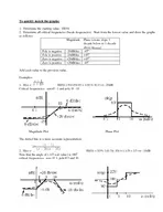
Where do the Bode diagram lines comes from 1 Determine the Transfer Function of the system 2 Rewrite it by factoring both the numerator and denominator into the standard form sp Kz where the s are called zeros and the s are called poles 3 Replace wi ID: 22582

Where the Bode

Share:

Link:

Embed:

Download Presentation from below link

Download Pdf The PPT/PDF document "Introduction to Bode Plot plots both ha..." is the property of its rightful owner. Permission is granted to download and print the materials on this web site for personal, non-commercial use only, and to display it on your personal computer provided you do not modify the materials and that you retain all copyright notices contained in the materials. By downloading content from our website, you accept the terms of this agreement.


Presentation Transcript

Introduction to Bode Plot 2 plots – both have logarithm of frequency on x- yaxis magnitude of transfer function, H(s), in dB yaxis phase angle The plot can be used to interpret how the input affects the output in both magnitude and phase over frequency. Where do the Bode diagram lines comes from? 1) Determine the Transfer Function of the system: ()()(1szs+= 2) Rewrite it by factoring both the numerator and denominator into the standard form ))(111+=s where the zs are called zeros and the p s are called poles. 3) Replace swith j. Then find the Magnitude of the Transfer F ))(111+=If we take the log10 of this magnitude and multiply it by 20 it takes on the form of 20 log10 (H(jw)) = ÷÷øöççèæ+)11110= )101011011011010---+++jw ach of these individual terms is very easy to show on a logarithmic plot. The entire Bode log magnitude plot is the result of the superposition of all the straight line terms This means with a little practice, we can quickly sketch the effect of each term and quickly fin d the overall effect. To do this we have to understand the effect of the different types of terms. These include: 1) Constant terms 2) Poles and Zeros at the origin | j | 3) Poles and Zeros not at the origin 1por 1 4) Complex Poles and Zeros (addressed later) Effect of Constant Terms: terms such as K contribute a straight horizontal line of magnitude 20 log10 = K Effect of Individual Zeros and Poles at the origin: A zeroat the origin occurs when there is an or j multiplying the numerator. Each occurrence of this causes a positively sloped line passing through ? = 1 with a rise of 20 db over a decade. = | w j | A pole at the origin occurs when there are s or multiplying the denominator. Each occurrence of this causes a negatively sloped line passing through ? = 1 with a drop of 20 db over a decade. = w Effect of Individual Zeros and Poles Not at the Origin Zeros and Poles not at the origin are indicated by the (1+ and (1+. The values and p in each of these expression is called a critical frequency (or break frequency). Below their criticalfrequency these terms do not contribute to the log magnitude of the overall plot. Above the critical y, they represent a ramp function of 20 db per decade. Zeros give a positive slope. Poles produce a negative slope. = iiw+1 20 log10 0.1 1 10 100 (log scale) 20 log10 ? 0.1 1 10 100 scale) 20 log(H -20 db dec. dec. +20 db z p20 db ? 0.1 1 10 100 (log scale) 20 log(H dec ? 0.1 1 10 100 (log scale) 20 log(H 20 db dec · To complete the log magnitude vs. frequency plot of a Bode diagram, we superposition all the lines of the different terms on the same plot. Example 1: For the transfer function given, sketch the Bode log magnitude diagram which shows how the log magnitude of the system is affected by changing input frequency. (TF=transfer function) + Step 1: Repose the equation in Bode plot form: 1 100 1 50 + recognized as 1 1 + with K = 0.01 and p1 = 50 For the constant, K: 20 log10(0.01) = - For the pole, with critical frequency, p Example 2: Your turn. Find the Bode log magnitude plot for the transfer function, 2 50 Start by simplifying the transfer function form: 50 0db ? (log scale) 20 log10 e 2 Solution:Your turn. Find the Bode log magnitude plot for the transfer function, 2 50 Simplify transfer function form: 4 Recognize: = 20 à 20 log10(20) = 26.02 1 zero at the origin 2 poles: at p = 5 and p Technique to get started: 1) Draw the line of each individual term on the graph 2) Follow the combined polezero at the origin line back to the left side of the graph. 3) Add the constant offset, 20 log10 to the value where the poleat the origin line intersects the left side of the graph.4) Apply the effect of the poles/zerosat the origin. working from left (low values) to right (higher values) of the poles/zeros. ? (log scale) Example 3: One more time. This one is harder. Find the Bode log magnitude plot for the transfer function, Simplify transfer function form: 0 db 4 0 db 10 8 0 db 8 0 db 40 db 10 10 10 20 (log scale) ? (log scale) Technique to get started: 1) Draw the line of each individual term on the graph 2) Follow the combined zero at the origin line back to the left side of the graph. 3) Add the constant offset, 20 log10 to the value where the poleat the origin line intersects the left side of the graph. 4) Apply the effect of the poles/zerosat the origin. working from left (low values) to right (higher values) of the poles/zeros. Example 3 Solution: Find the Bode log magnitude plot for the transfer function, Simplify transfer function form: Recognize: K = 100 20 log10(100) = 40 1 at the origin 1 zero at z = 20 2 poles: at p = 0.5 and p 0 db 4 0 db 10 8 0 db 8 0 db 4 0 db 10 10 10 20 20 40 ? (log scale) Technique to get started: 1) Draw the line of each individual term on the graph 2) Follow the combined polezero at the origin line back to the left side of the graph. 3) Add the constant offset, 20 log10 to the value where the poleat the origin line intersects the left side of the graph. 4) Apply the effect of the poles/zerosat the origin. working from left (low values) to right (higher values) of the poles/zeros. The plot of the log magnitude vs. input frequency is only half of the story. We also need to be able to plot the phase angle vs. input frequency on a log scale as well to complete the full Bode diagram.. For our original transfer function, ))(111+=he cumulative phase angle associated with this function are given by ))(111ÐÐÐÐThen the cumulative phase angle as a function of the input frequency may be written as ûùêëé---+++)())(111 Once again, to show the phase plot of the Bode diagram, lines can be drawn for each of the different terms. the total effect may be found by superposition. Effect of Constants on Phase: positive �0, s no effect on phase. A negative constant, K will set up a phase shift of ±180(Remember real vs imaginary plots – a negative real number is at ±180o relative to the origin) Effect of Zeros at the origin on Phase Angle: Zeros at the origin, cause a constant +90 degree shift for each zero. Effect of Poles at the origin on Phase Angle: at the origin, a constant 90 degree shift for each pole. (log) +90 deg ? 90 deg Effect of Zeros not at the origin on Phase Angle: Zeros not at the origin, like 1 have no phase shift for frequencies much lower than z, have a + 45 deg shift at z, and have a +90 deg shift for frequencies much higher than z . To draw the lines for this type of term, the transition from 0o to +90o is drawn over 2 decades, starting at 0.1 and ending at 10z Effect of Poles not at the origin on Phase Angle: Poles not at the origin, like 11p have no phase shift for frequencies much lower than p, have a -45 deg shift at p, and have a -90 deg shift for frequenciesmuch higher than p . To draw the lines for this type of term, the transition from 0o to - is drawnver 2 decades, starting at 0.1p and ending at 10p When drawing the phase angle shift for no-origin zeros and poles, first locate the critical frequency of the zero or pole. Then start the transition 1 decade before, following a slope of /decade. Continue the transition until reaching the frequency one decade past the critical frequency. Now let’s complete the Bode Phase diagrams for the previous examples: ? 1 10100 +90 deg +45 deg 0.1p 1p 10p100p -90 deg 45 deg Example 1: For the Transfer Function given, sketch the Bode diagram which shows how the phase of the system is affected by changing input frequency. 50 s + 20 log|TF 50 5 500 rad/s ? ? 0.5 Example 2Repeat for the transfer function, | 4250 ? (log scale) ? (log scale) 20 log10 Phase Angle Example 2 Solution:Repeat for the transfer function, | 4250 0 db 4 0 db 10 8 0 db 8 0 db 4 0 db 10 10 10 ? (log scale) ? (log scale) 20 log10 Phase Angle Example 3: Find the Bode log magnitude and phase angle plot for the transfer function, 10 200 s+ 0 db 4 0 db 10 8 0 db 8 0 db 4 0 db 10 10 10 ? (log scale) ? (log scale) 20 log10 Phase Angle Example 3: Find the Bode log magnitude and phase angle plot for the transfer function, 10 200 s+ 0 db 4 0 db 10 8 0 db 8 0 db 4 0 db 10 10 10 ? (log scale) ? (log scale) 20 log10 Phase Angle Example 4 Sketch the Bode plot (Magnitude and Phase Angle) for | Angle of TF Example 4 Sketch the Bode plot (Magnitude and Phase Angle) for = 10 1 Therefore: K = 10 so 20log10(10) = 20 db One zero: z = 1 Two poles: p = 10 and p = 1000 | Angle of TF 20 0 db - - 90 0 deg - - Matlab can also be used to draw Bode plots: (with the sketched Bode Plot superimposed on the actual plot) 1,5,100); %setup for x- %transfer function %transfer function converted to dB %phase done in radians %phase done in degrees %semilog plot xlabel('frequency [rad/s]'),ylabel('20 log10(|TF|) [db]'),grid %xaxis label xlabel('frequency [rad/s]'),ylabel('Phase Angle [deg]'),grid 10 -10 20 30 40 frequency [rad/s] 20 log10(|TF|) [db] 10 100 frequency [rad/s] Phase Angle [deg] Notice that the actual plot does not follow the sketched plot exactly. There is error between our sketched method and the actual Bode plot. How much error is expected?Let’s look at an example of a zero, ) =. Note, ? = 10 rad/s The largest error that occurs on the Magnitude plot is right at the critical frequency. It is on the order of 3 db. 20 30 40 50 frequency [rad/s] 20 log10(|TF|) [db] 10 40 60 80 100 frequency [rad/s] Phase Angle [deg] The largest error that is shown on the Phase plot occurs at 0.1? and 10? (one decade above and below the critical frequency). Error at these points is about 6 degrees. It’s understood that sketching the Bode diagrams will contain some error but this is generally considered acceptable practice. To quickly sketch the graphs: 1. Determine the starting value: |2. Determine all critical frequencies (break frequencies). Start from the lowest value and draw the graphs as follows: Magnitude Phase (create slope 1 decade below to 1 decade above w Pole is negative Pole is positive Zero is negative Zero is positive Add each value to the previous value. 1. H(s) = |H(0)| = |0+1/0+10 = 1/10 |= |� = -tical frequencies: zero@ -1 and pole @ - Magnitude Plot Phase Plot The dotted line is a more accurate representation. 2. H(s) = |H(0)| = |10*(-10) |= |-�1/3| = 1/3 = -Note that the angle of (-1/3 real value) is 180ocritical frequencies: zero @ 1, pole@3 and 10