/
Lecture  Variants of the LMS algorithm Standard LMS Algorithm FIR lters Lecture  Variants of the LMS algorithm Standard LMS Algorithm FIR lters

Lecture Variants of the LMS algorithm Standard LMS Algorithm FIR lters - PDF document

luanne-stotts
luanne-stotts . @luanne-stotts
Follow
646 views
Uploaded On 2014-12-24

Lecture Variants of the LMS algorithm Standard LMS Algorithm FIR lters - PPT Presentation

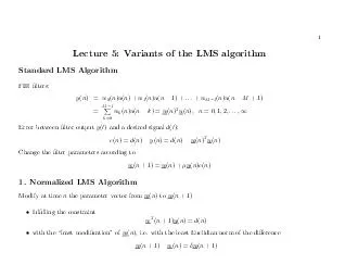
1 0 n 0 Error between 64257lter output and a desired signal Change the 64257lter parameters according to 1 57525u 1 Normalized LMS Algorithm Modify at time the parameter vector from to 1 ful64257lling the constraint 1 with the least modi6425 ID: 28975

algorithm lms step 64257 lms algorithm 64257 step page 8722 lecture5 adaptation error sign size 64256 time 57525 947

Share:

Link:

Embed:

Download Presentation from below link

Download Pdf The PPT/PDF document "Lecture Variants of the LMS algorithm S..." is the property of its rightful owner. Permission is granted to download and print the materials on this web site for personal, non-commercial use only, and to display it on your personal computer provided you do not modify the materials and that you retain all copyright notices contained in the materials. By downloading content from our website, you accept the terms of this agreement.


Presentation Transcript

Lecture5 2nŠi))u(nŠi)d(nŠ1i=0wi(n)u(nŠi 2MŠ1i=0(u(nŠi))2=(n)Š MŠ1i=0wi(n)u(nŠi)) MŠ1i=0(u(nŠi))2=2e(n) Thus,theminimumofthecriterion +1))willbeobtainedusingtheadaptationequation+1)= Inordertoaddanextrafreedomdegreetotheadaptationstrategy,oneconstant,,controllingthestepsizewillbeintroduced:+1)=)+ MŠ1i=0(u(nŠi))2e(n)u(nŠjj(nµ u Toovercomethepossiblenumericaldicultieswhen isveryclosetozero,aconstant0isused: +1)= a+u (n)2e(n)u(nŠj) ThisistheupdatingequationusedintheNormalizedLMSalgorithm. Lecture5ComparisonofLMSandNLMSwithintheexamplefromLecture4(channelequalization) 500 1000 1500 2000 250 0 103 102 101 100 Learning curve Ee2(n) for LMS algorithmtime step n =0.075 µ=0.025 µ=0.0075 500 1000 1500 2000 250 0 103 102 101 100 101 Learning curve Ee2(n) for Normalized LMS algorithmtime step n =1.5 µ=1.0 µ=0.5 µ=0.1 Lecture52.LMSAlgorithmwithTimeVariableAdaptationStepHeuristicsofthemethod:Wecombinethebene“tsoftwodierentsituations:TheconvergencetimeconstantissmallforlargeThemean-squareerrorinsteadystateislowforsmallTherefore,intheinitialadaptationstagesiskeptlarge,thenitismonotonicallyreduced,suchthatinthe“naladaptationstageitisverysmall.Therearemanyreceiptsofcoolingdownanadaptationprocess.Monotonicallydecreasingthestepsize Disadvantagefornon-stationarydata:thealgorithmwillnotreactanymoretochangesintheoptimumsolution,forlargevaluesofVariableStepalgorithm: +1)= (n(n)u (n)e(n)whereM(n µ0(n00µ1(n).00Š1(n)  Lecture5ComparisonofLMSandvariablesizeLMS( )withintheexamplefromLecture4(channelequalization)=[10;20;50] 500 1000 1500 2000 2500 103 102 101 100 2(n) for LMS algorithmtime step n =0.075 µ=0.025 µ=0.0075 500 1000 1500 2000 2500 103 102 101 100 101 2(n) for variable size LMS algorithmtime step n c=20 LMS µ=0.0075 Lecture5Veryfastcomputation:ifisconstrainedtotheform,onlyshiftingandadditionoperationsareDrawback:theupdatemechanismisdegraded,comparedtoLMSalgorithm,bythecrudequantizationofgradientestimates.*Thesteadystateerrorwillincrease*TheconvergenceratedecreasesThefastestofthem,Sign-Sign,isusedintheCCITTADPCMstandardfor32000bpssystem. Lecture54.LinearsmoothingofLMSgradientestimatesLowpass“lteringthenoisygradientLetusrenamethenoisygradient (nw Jg (nw J=Š2u Passingthesignals)throughlowpass“lterswillpreventthelarge”uctuationsofdirectionduringadaptationprocess.LPFwhereLPFdenotesalowpass“lteringoperation.Theupdatingprocesswillusethe“lterednoisygradient +1)= (n)Šµb Thefollowingversionsarewellknown:AveragedLMSalgorithmWhenLPFisthe“lterwithimpulseresponse(0)= 1)= +1)=weobtainsimplytheaverageofgradientcomponents: +1)= (n Nnj=nŠN+1e(j)u (j) Lecture55.NonlinearsmoothingofLMSgradientestimatesIfthereisanimpulsiveinterferenceineither)or),theperformancesofLMSalgorithmwilldrasticallydegrade(sometimesevenleadingtoinstabilty).Smoothingthenoisygradientcomponentsusinganonlinear“lterprovidesapotentialsolution.TheMedianLMSAlgorithmComputingthemedianofwindowsize+1,foreachcomponentofthegradientvector,willsmoothouttheeectofimpulsivenoise.Theadaptationequationcanbeimplementedas+1)=*Experimentalevidenceshowsthatthesmoothingeectinimpulsivenoiseenvironmentisverystrong.*Iftheenvironmentisnotimpulsive,theperformancesofMedianLMSarecomparablewiththoseofLMS,thustheextracomputationalcostofMedianLMSisnotworth.*However,theconvergenceratemustbeslowerthaninLMS,andtherearereportsofinstabiltyoccurringwhithMedianLMS. Lecture57.LMSVolterraalgorithmWewillgeneralizetheLMSalgorithm,fromlinearcombinationofinputs(FIR“lters)toquadraticcombina-tionsoftheinputs. (n)Tu )Linearcombinerbinerk(n)u(nŠk)+MŠ1i=0MŠ1j=iw[2]i,j(n)u(nŠi)u(nŠj)(3)QuadraticcombinerWewillintroducetheinputvectorwithdimension+1) ...u+1)...u+1)andtheparametervector 0(n)w[1]1(n)...wwMŠ1(n)w[2]0,0(n)w[2]0,1(n)...wwMŠ1,MŠ1(n)TNowtheoutputofthequadratic“lter(3)canbewritten (n)T andthereforetheerror (n)T isalinearfunctionofthe“lterparameters(i.e.theentriesof (n)) Lecture5andtheadaptationproblemdecouplesintwoproblems,i.e.theWieneroptimal“lterswillbesolutions n)u n)R4w n)u (n)andsimilarly,theLMSsolutionscanbeanalyzedseparately,forlinear, ,andquadratic, ,coe-cients,accordingtotheeigenvaluesof