/
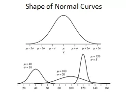
Shape of Normal Curves Shape of Normal Curves Shape of Normal Curves Shape of Normal Curves

Shape of Normal Curves Shape of Normal Curves - PowerPoint Presentation

luanne-stotts
luanne-stotts . @luanne-stotts
Follow
393 views
Uploaded On 2018-02-28

Shape of Normal Curves Shape of Normal Curves - PPT Presentation

6895997 Rule Areas under Normal Curve Areas under Normal Curvecont Example Normal Distribution The brain weights of adult Swedish males are approximately normally distributed with mean μ 1400 g and standard deviation ID: 638942

distribution normal swedish brain normal distribution brain swedish qqplots population adult evidence nonnormality sas skewed cont 100 probability male

Share:

Link:

Embed:

Download Presentation from below link

Download Presentation The PPT/PDF document "Shape of Normal Curves Shape of Normal C..." is the property of its rightful owner. Permission is granted to download and print the materials on this web site for personal, non-commercial use only, and to display it on your personal computer provided you do not modify the materials and that you retain all copyright notices contained in the materials. By downloading content from our website, you accept the terms of this agreement.


Presentation Transcript

Slide1

Shape of Normal CurvesSlide2

Shape of Normal CurvesSlide3

68%-95%-99.7% RuleSlide4

Areas under Normal CurveSlide5

Areas under Normal Curve(cont)Slide6

Example: Normal Distribution

The brain weights of adult Swedish males are

approximately

normally distributed with mean μ = 1,400 g and standard deviation

= 100 g. (No real life population follows a normal distribution

exactly!

)

a) What is the probability that an adult Swedish male has a brain weight of less then 1,500 g?

b) What is the probability that an adult Swedish male has a brain weight between 1,475 g and 1,600 g?Slide7

Example: Normal Distribution (cont)

μ = 1,400 g and

= 100 g

a) What is the probability that an adult Swedish male has a brain weight of less then 1,500 g?Slide8

Example: Normal Distribution (cont)

μ = 1,400 g and

= 100 g

b) What is the probability that an adult Swedish male has a brain weight between 1,475 g and 1,600 g?Slide9

Area under the normal curve above Slide10

Example: Normal Distribution

The brain weights of adult Swedish males are

approximately

normally distributed with mean μ = 1,400 g and standard deviation

= 100 g. (No real life population follows a normal distribution

exactly!

)

c) What is the 55

th

percentile for the distribution of brain weights? Slide11

Example (ExDispersion.sas)

Determine the percentage of data points within 1 SD? 2 SD?

7

21

12

4

16

12

10

13

6

13

13

13

12

18

15

16

3

6

9

11Slide12

Example: Normality (ExNormal.sas)

7

21

12

4

16

12

10

13

6

13

13

13

12

18

15

16

3

6

9

11Slide13

Example:

QQPlots

– Normal (ExQQplot.sas)Slide14

Example:

QQPlots

– Right SkewedSlide15

Example: QQPlots

– Left SkewedSlide16

Example: QQPlots

– Long TailSlide17

Example: QQPlots

– Tails?Slide18

Example 4.4.5: Nonnormal

DataSlide19

Interpretation of Shapiro-Wilk Test

P-Value

Interpretation

< 0.001

Very strong evidence for nonnormality

< 0.01

Strong evidence for nonnormality

< 0.05

Moderate evidence for nonnormality

< 0.10

Mild or weak evidence for nonnormality

 0.10

No compelling

evidence for nonnormalitySlide20

Objective Measure: SAS

Tests for Normality

Test

Statistic

p Value

Shapiro-

Wilk

W

0.98762

Pr < W

0.8757

Kolmogorov

-Smirnov

D

0.092489

Pr > D

>0.1500

Cramer-von

Mises

W-Sq

0.042289

Pr > W-Sq

>0.2500

Anderson-Darling

A-Sq

0.233462

Pr > A-Sq

>0.2500Slide21

Objective Measure: SAS

Tests for Normality

Test

Statistic

p Value

Normal

W

0.98762

Pr < W

0.8757

Right

Skewed

W

0.949844

Pr >

W

0.4226

Left Skewed

W

0.925624

Pr >

W

0.0479

Long

Tailed

W

0.927118

Pr >

W

0.0043

Short Tailed

W

0.949227

Pr > W

0.0317Slide22

Example: QQPlots

xSlide23

Example 4.10: Continuity Correction

Table 4.1 shows the distribution of litter size for a population of female mice with population mean 7.8 and SD 2.3.

xSlide24

Example 4.10: Continuity Correction(cont)

Table 4.1 shows the distribution of litter size for a population of female mice with population mean 7.8 and SD 2.3.

x