/
0 + 0 +

0 + - PowerPoint Presentation

marina-yarberry
marina-yarberry . @marina-yarberry
Follow
366 views
Uploaded On 2016-02-23

0 + - PPT Presentation

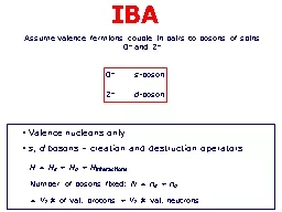
s boson 2 d boson Valence nucleons only s d bosons creation and destruction operators H H s H d H interactions Number of bosons fixed ID: 227817

energies 000 00000 iba 000 energies iba 00000 2000 bosons group structure nuclei 0000 8000 triangle hamiltonian boson number

Share:

Link:

Embed:

Download Presentation from below link

Download Presentation The PPT/PDF document "0 +" is the property of its rightful owner. Permission is granted to download and print the materials on this web site for personal, non-commercial use only, and to display it on your personal computer provided you do not modify the materials and that you retain all copyright notices contained in the materials. By downloading content from our website, you accept the terms of this agreement.


Presentation Transcript

Slide1

0+ s-boson2+ d-boson

Valence nucleons only s, d bosons – creation and destruction operators H = Hs + Hd + Hinteractions Number of bosons fixed: N = ns + nd = ½ # of val. protons + ½ # val. neutrons

IBA

Assume valence

fermions couple in pairs

to

bosons of spins 0

+

and 2

+Slide2

IBA Models IBA – 1 No distinction of p, n

IBA – 2 Explicitly write p, n parts IBA – 3, 4 Take isospin into account p-n pairs IBFM Int. Bos. Fermion Model Odd A nuclei

H = He – e

+ Hs.p. + Hint core IBFFM Odd – odd nuclei

[ (f, p) bosons for  = - states spdf IBA ]

Parameters

Different models have different numbers of parameters. Be careful in evaluating/comparing different models. Be alert for hidden parameters. Lots of parameters are not necessarily bad – they may be mandated by the data, but look at them with your eyes open.Slide3

F. Iachello and A. Arima, The Interacting Boson Model (Cambridge University Press, Cambridge, England, 1987).F. Iachello and P. Van Isacker, The Interacting Boson-Fermion Model (Cambridge University Press, Cambridge, England, 2005) R.F. Casten and D.D. Warner, Rev. Mod. Phys. 60

(1988) 389.R.F. Casten, Nuclear Structure from a Simple Perspective, 2nd Edition (Oxford Univ. Press, Oxford, UK, 2000), Chapter 6 (the basis for most of these lectures).D. Bonatsos, Interacting boson models of nuclear structure, (Clarendon Press, Oxford, England, 1989)Many articles in the literatureBackground, ReferencesSlide4

That relation is based on the operators that create, destroy s and d bosonss†, s, d†

, d operators Ang. Mom. 2d† , d  = 2, 1, 0, -1, -2Hamiltonian is written in terms of s, d

operatorsSince boson number is conserved

for a given nucleus,

H can only contain “bilinear” terms: 36 of them.s†s, s†d, d†s, d†dGr. Theor. classification of Hamiltonian

IBA has a deep relation to Group theoryGroup is calledU(6) Slide5

OK, here’s what you need to remember from the Group TheoryGroup Chain: U(6)  U(5)  O(5)  O(3)A dynamical symmetry corresponds to a certain structure/shape of a nucleus and its characteristic excitations. The IBA has three dynamical symmetries: U(5), SU(3), and O(6).

Each term in a group chain representing a dynamical symmetry gives the next level of degeneracy breaking. Each term introduces a new quantum number that describes what is different about the levels.These quantum numbers then appear in the expression for the energies, in selection rules for transitions, and in the magnitudes of transition rates.Slide6

Concept of a Dynamical Symmetry

NOK, here’s the key point :Spectrum generating algebra !!Slide7

Group theory of the IBA U(6) 36 generators conserve N U(5) 25 generators conserve ndSuppose:

H = α1 CU(6) + α2 CU(5) (1)All states of a given nucleus have same N. So, if α2 = 0, i.e., H = α1 CU(6) only, then all states would be degenerate.

But these states have different nd. Thus, if we consider the full eq. 1, then the degeneracy is broken because C

U(5)

gives E = f (nd). In group notation Dyn.Symm.

U(6)  U(5)  … Recall: O(3)  O(2)Slide8

Group Structure of the IBAs boson :d boson :U(5)

vibratorSU(3)rotorO(6)γ-soft15

U(6)

Sph.

Def.

Magical group theory stuff happens hereSymmetry Triangle of the IBASlide9

Classifying Structure -- The Symmetry Triangle Most nuclei do not exhibit the idealized symmetries but rather lie in transitional regions. Mapping the triangle.

Sph.DeformedSlide10

Most general IBA Hamiltonian in terms with up to four boson operators (given N)

IBA HamiltonianMixes d and s components of the wave functionsd+dCounts the number of d bosons out of N bosons, total. The rest are s-bosons: with Es = 0 since we deal only with excitation energies. Excitation energies depend ONLY on the number of d-bosons. E(0) = 0, E(1) = ε , E(2) = 2 ε.

Conserves the number of d bosons. Gives terms in the Hamiltonian where the energies of configurations of 2 d bosons depend on their total combined angular momentum. Allows for anharmonicities in the phonon multiplets.

dSlide11

U(5)Spherical, vibrational nucleiSlide12

What J’s? M-scheme Look familiar? Same as quadrupole vibrator.U(5) also includes anharmonic spectra6+, 4+

, 3+, 2+, 0+4+, 2+, 0+2+0+ 3 2 1 0nd

Simplest Possible

IBA Hamiltonian –

given by energies of the bosons with NO interactionsExcitation energies so, set s = 0, and drop subscript d on d

What is spectrum? Equally spaced levels defined by number of d bosons= E of d bosons + E of s bosonsSlide13

E2 Transitions in the IBA Key to most tests Very sensitive to structure

E2 Operator: Creates or destroys an s or d boson or recouples two d bosons. Must conserve NT = e Q = e[s† + d†s + χ (d† )(2)]

Specifies relative strength of this termSlide14

E2 transitions in U(5)χ = 0That is: T = e[s† + d†s] Why? So that it can create or destroy a single d boson, that is, a single phonon.6

+, 4+, 3+, 2+, 0+4+, 2+, 0+2+0+ 3 2 1 0ndSlide15

Creation and destruction operators asExample: Consider the case we have just discussed – the spherical vibrator.

024,2,00E2E

12

Why is the B(E2: 4 – 2) = 2 x B(E2: 2– 0)

??Difficult to see with Shell Model wave functions with 1000’s of componentsHowever, as we have seen, it is trivial using destruction operators

WITHOUT EVER KNOWING ANYTHING ABOUT THE DETAILED STRUCTURE OF THESE VIBRATIONS !!!! These operators give the relationships between states.“Ignorance operators”Slide16

0

+2+6+. . .8+. . .

Vibrator (H.O.)

E(I)

= n ( 

0 ) R4/2= 2.0

VibratorSlide17
Slide18

Deformed nucleiUse the same Hamiltonian but re-write it in more convenient and physically intuitive formSlide19

IBA Hamiltonian

Complicated and, for many calculations, not really necessary to use all these terms and all 6 parametersTruncated form with just two parameters – RE-GROUP and keep some of the terms above.H = ε nd -  Q  Q Q = e[s† + d†s + χ (d†

)(2)]

Competition:

ε nd term gives vibrator.  Q  Q term gives deformed nuclei.

More complicated forms exist but this is the form we will use. It works extremely well in most cases.Slide20

Relation of IBA Hamiltonian to Group Structure

We will see later that this same Hamiltonian allows us to calculate the properties of a nucleus ANYWHERE in the triangle simply by choosing appropriate values of the parameters= -1.32Slide21

In a region of increasing g softness, can simulate simply by decreasing |c| towards zeroSlide22

SU(3)Deformed nucleiSlide23

Any calculation deviating from U(5) gives wave functions where nd is no longer a good quantum number. If the wave function is expressed in a U(5) – vibrator – basis, then it contains a mixture of terms. Understanding these admixtures is crucial to understanding IBA calculations

Wave functions in SU(3): Consider non-diagonal effects of the QQ term in H on nd components in the wave functionsQ operator: Q = (s† d + d †s) + (d † d )(2)QQ = [ { (s† d + d †s) + χ(

d †d ) (2) } x { (s

d + d †s) + (d †d )(2) } ] ~ s† d

s† d + s† d d †s + s† d d

d ….

D

n

d

= -2 0 -1 …. 2, 0, 1 Slide24

MSlide25

Typical SU(3) Scheme SU(3)  O(3)

K bands in (, ) : K = 0, 2, 4, - - - - 

Characteristic signatures: Degenerate bands within a group

Vanishing B(E2) values between groups

Allowed transitions between bands within a group Where? N~ 104, Yb, HfSlide26

Totally typical exampleSimilar in many ways to SU(3). But note that the two excited excitations are not degenerate as they should be in SU(3). While SU(3) describes an axially symmetric rotor, not all rotors are described by SU(3) – see later discussionSlide27

O(6)Axially asymmetric nuclei(gamma-soft)Slide28
Slide29
Slide30

Note: Uses χ = 0Slide31

196Pt: Best (first) O(6) nucleus -softSlide32

Thus far, we have only dealt with nuclei corresponding to one of the three dynamical symmetries. Probably <1% of nuclei do that. So, how do we treat the others? That is, how do we calculate with the IBA AWAY from the vertices of the symmetry triangle? A couple of interesting examples first, then a general approach --- The technique of Orthogonal Crossing Contours (OCC)More General IBA calculations

c Slide33

CQF along the O(6) – SU(3) leg H = -κ Q • Q

Only a single parameter,  H = ε nd -  Q  Q Two parametersε / and 

We will discuss 1) and 4). The others are included in the slides in the AppendixSlide34

c H = ε nd -  Q  Q

ε = 0

/ε 168-Er very simple 1-parameter calculationH = -  Q  Q

is just scale factorSo, only parameter is cSlide35

1Slide36
Slide37

Mapping the Entire Triangle 2 parameters2-D surface

cH = ε nd -

 Q  Q

Parameters:

, c (within Q) /ε

/ε /ε Problem: varies from zero to infinity: Awkward. So, introduce a simple change of variablesSlide38

Spanning the TriangleH = c [

ζ ( 1 – ζ ) nd 4NB Qχ ·Qχ -

]

ζ

χ

U(5)

0

+

2

+

0

+

2

+

4

+

0

2.0

1

ζ

= 0

O(6)

0

+

2

+

0

+

2

+

4

+

0

2.5

1

ζ

= 1,

χ

= 0

SU(3)

2

γ

+

0

+

2

+

4

+

3.33

1

0

+

0

ζ

= 1,

χ

= -1.32Slide39

23

5Slide40

H has two parameters. A given observable can only specify one of them. What does this imply? An observable gives a contour of constant values within the triangle

= 2.9R4/2Slide41

At the basic level : 2 observables (to map any point in the symmetry triangle)Preferably with perpendicular trajectories in the triangleA simple way to pinpoint structure. Technique of Orthogonal Crossing Contours (OCC)

Simplest Observable: R4/2Only provides a locus of structure3.33.12.92.72.52.2Slide42

Contour Plots in the Triangle3.33.1

2.92.72.52.2R4/22.247

1310

17

2.24710

13170.1

0.05

0.01

0.4Slide43

We have a problemWhat we have:

Lots of What we need:

Just one

+2.9

+2.0

+1.4

+0.4

+0.1

-0.1

-0.4

-1

-2.0

-3.0

Fortunately:Slide44

Vibrator

Rotorγ - softMapping Structure with Simple Observables – Technique of Orthogonal Crossing Contours

Burcu Cakirli et al.

Beta decay exp. + IBA calcs.Slide45

Evolution of StructureComplementarity of macroscopic and microscopic approaches. Why do certain nuclei exhibit specific symmetries? Why these evolutionary trajectories?

What will happen far from stability in regions of proton-neutron asymmetry and/or weak binding?Slide46

Special Thanks to: Franco Iachello Akito Arima Igal Talmi Dave Warner Peter von Brentano Victor Zamfir

Jolie Cizewski Hans Borner Jan Jolie Burcu Cakirli Piet Van Isacker Kris Heyde Many othersSlide47

Appendix: Trajectories-by-eye Running the IBA program using the Titan computer at Yale Examples “2” and “3” skipped earlier of the use of the CQF form of the IBASlide48

Trajectories at a Glance

R4/2Slide49

Nuclear Model Codes at YaleComputer name: Titan Connecting to SSH: Quick connectHost name: titan.physics.yale.eduUser name: phy664Port Number 22Password: nuclear_codescd phintmpico filename.in

(ctrl x, yes, return)runphintm filename (w/o extension)pico filename.out (ctrl x, return)Slide50

Input $diag eps = 0.20, kappa = 0.00, chi =-0.00, nphmax = 6, iai = 0, iam = 6, neig = 3, mult=.t.,ell=0.0,pair=0.0,oct=0.0,ippm=1,print=.t. $

$em E2SD=1.0, E2DD=-0.00 $ SLCT 2 2+ 0+ 2 99999 Output---------------------------L P = 0+ Basis vectors |NR> = |ND,NB,NC,LD,NF,L P> --------------------------- | 1> = | 0, 0, 0, 0, 0, 0+> | 2> = | 2, 1, 0, 0, 0, 0+> | 3> = | 3, 0, 1, 0, 0, 0+> | 4> = | 4, 2, 0, 0, 0, 0+> | 5> = | 5, 1, 1, 0, 0, 0+> | 6> = | 6, 0, 2, 0, 0, 0+> | 7> = | 6, 3, 0, 0, 0, 0+>

Energies 0.0000 0.4000 0.6000 0.8000 1.0000 1.2000 1.2000

Eigenvectors

1: 1.000 0.000 0.000 2: 0.000 1.000 0.000 3: 0.000 0.000 1.000 4: 0.000 0.000 0.000 5: 0.000 0.000 0.000 6: 0.000 0.000 0.000 7: 0.000 0.000 0.000

---------------------------L P = 1+No states---------------------------L P = 2+ Energies 0.2000 0.4000 0.6000 0.8000 0.8000 1.0000 1.0000 1.2000 1.2000---------------------------L P = 3+

Energies

0.6000 1.0000 1.2000

---------------------------

L P = 4+

Energies

0.4000 0.6000 0.8000 0.8000 1.0000 1.0000 1.2000 1.2000 1.2000

---------------------------

L P = 5+

Energies

0.8000 1.0000 1.2000

---------------------------

L P = 6+

Energies

0.6000 0.8000 1.0000 1.0000 1.2000 1.2000 1.2000

--------------------------

Transitions: 2+ -> 0+ (BE2)

2+,1 -> 0+,1: 6.00000 2+,1 -> 0+,2: 2.00000 2+,1 -> 0+,3: 0.00000

2+,2 -> 0+,1: 0.00000 2+,2 -> 0+,2: 0.00000 2+,2 -> 0+,3: 2.40000

2+,3 -> 0+,1: 0.00000 2+,3 -> 0+,2: 5.60000 2+,3 -> 0+,3: 0.00000

and 0+ -> 2+ (BE2)

0+,1 -> 2+,1: 30.00000 0+,2 -> 2+,1: 10.00000 0+,3 -> 2+,1: 0.00000

0+,1 -> 2+,2: 0.00000 0+,2 -> 2+,2: 0.00000 0+,3 -> 2+,2: 12.00000

0+,1 -> 2+,3: 0.00000 0+,2 -> 2+,3: 28.00000 0+,3 -> 2+,3: 0.00000

Transitions: 4+ -> 2+ (BE2)

4+,1 -> 2+,1: 10.00000 4+,1 -> 2+,2: 0.00000 4+,1 -> 2+,3: 2.28571

4+,2 -> 2+,1: 0.00000 4+,2 -> 2+,2: 6.28571 4+,2 -> 2+,3: 0.00000

4+,3 -> 2+,1: 0.00000 4+,3 -> 2+,2: 0.00000 4+,3 -> 2+,3: 3.85714

U(5)

Basis

Energies

Pert.

Wave

Fcts.Slide51

Input $diag eps = 0.0, kappa = 0.02, chi =-0.0, nphmax = 6, iai = 0, iam = 6, neig = 5, mult=.t.,ell=0.0,pair=0.0,oct=0.0,ippm=1,print=.t. $

$em E2SD=1.0, E2DD=-0.00 $ 99999 Output---------------------------L P = 0+ Basis vectors |NR> = |ND,NB,NC,LD,NF,L P> --------------------------- | 1> = | 0, 0, 0, 0, 0, 0+> | 2> = | 2, 1, 0, 0, 0, 0+> | 3> = | 3, 0, 1, 0, 0, 0+> | 4> = | 4, 2, 0, 0, 0, 0+> | 5> = | 5, 1, 1, 0, 0, 0+> | 6> = | 6, 0, 2, 0, 0, 0+> | 7> = | 6, 3, 0, 0, 0, 0+> Energies 0.0000 0.3600 0.5600 0.9200 0.9600 1.0800 1.2000

Eigenvectors 1: -0.433 0.000 0.685 0.000 0.559

2: -0.750 0.000 0.079 0.000 -0.581

3: 0.000 -0.886 0.000 0.463 0.000 4: -0.491 0.000 -0.673 0.000 0.296 5: 0.000 -0.463 0.000 -0.886 0.000 6: 0.000 0.000 0.000 0.000 0.000 7: -0.094 0.000 -0.269 0.000 0.512---------------------------L P = 1+No states---------------------------

L P = 2+ Energies 0.0800 0.2000 0.5600 0.6400 0.7600 0.8000 1.0400 1.1200 1.1600--------------------------L P = 3+ Energies 0.3600 0.9200 1.0800---------------------------L P = 4+

Energies

0.2000 0.3600 0.5600 0.7600 0.8000 0.9200 1.0800 1.1200 1.1600

--------------------------

L P = 5+

Energies

0.5600 0.8000 1.1200

---------------------------

L P = 6+

Energies

0.3600 0.5600 0.8000 0.9200 1.0800 1.0800 1.1200

---------------------------

Binding energy = -0.6000 , eps-eff = -0.1200

O(6)

Basis

Pert.

Wave

Fcts.

EnergiesSlide52

******************** Input file contents ******************** $diag eps = 0.00, kappa = 0.02, chi =-1.3229, nphmax = 6, iai = 0, iam = 6, neig = 5,

mult=.t.,ell=0.0,pair=0.0,oct=0.0,ippm=1,print=.t. $ $em E2SD=1.0, E2DD=-2.598 $ 99999 *************************************************************---------------------------L P = 0+ Basis vectors |NR> = |ND,NB,NC,LD,NF,L P> --------------------------- | 1> = | 0, 0, 0, 0, 0, 0+> | 2> = | 2, 1, 0, 0, 0, 0+> | 3> = | 3, 0, 1, 0, 0, 0+> | 4> = | 4, 2, 0, 0, 0, 0+> | 5> = | 5, 1, 1, 0, 0, 0+> | 6> = | 6, 0, 2, 0, 0, 0+>

| 7> = | 6, 3, 0, 0, 0, 0+> Energies

0.0000 0.6600 1.0800 1.2600 1.2600 1.5600 1.8000

Eigenvectors 1: 0.134 0.385 -0.524 -0.235 0.398 2: 0.463 0.600 -0.181 0.041 -0.069 3: -0.404 -0.204 -0.554 -0.557 -0.308 4: 0.606 -0.175 0.030 -0.375 -0.616 5: -0.422 0.456 -0.114 0.255 -0.432 6: -0.078 0.146 -0.068 0.245 -0.415 7: 0.233 -0.437 -0.606 0.606 0.057

---------------------------L P = 1+No states---------------------------L P = 2+

Energies

0.0450 0.7050 0.7050 1.1250 1.1250 1.3050 1.3050 1.6050

---------------------------

L P = 3+

Energies

0.7500 1.1700 1.6500

---------------------------

L P = 4+

Energies

0.1500 0.8100 0.8100 1.2300 1.2300 1.2300 1.4100 1.4100

---------------------------

L P = 5+

Energies

0.8850 1.3050 1.3050

---------------------------

L P = 6+

Energies

0.3150 0.9750 0.9750 1.3950 1.3950 1.5750 1.5750

---------------------------

Binding energy = -1.2000 , eps-eff = -0.1550

SU(3)

Wave fcts. in U(5) basisSlide53

“Universal” IBA Calculations for the SU(3) – O(6) leg H = -

κ Q • Q κ is just energy scale factor Ψ’s, B(E2)’s independent of κ Results depend only on χ [ and, of course, vary with N

B ]

Can plot any observable as a set of

contours vs. NB and χ. 2Slide54

Universal O(6) – SU(3) Contour Plots H = -κ Q • Q

χ = 0 O(6) χ = - 1.32 SU(3) SU(3)Slide55
Slide56

Systematics and collectivity of the lowest vibrational modes in deformed nucleiNotice that the the b mode is at higher energies (~ 1.5 times the g vibration near mid-shell)* and fluctuates more. This points to lower collectivity of the

b vibration.* Remember for later !Max. Coll.Increasing g softnessSlide57
Slide58
Slide59

Os isotopes from A = 186 to 192: Structure varies from a moderately gamma soft rotor to close to the O(6) gamma-independent limit. Describe simply with: H = -κ Q • Q  : 0

 small as A decreases3Slide60

End of Appendix

Related Contents


Next Show more