/
International Short Conference on Applied Coastal Research International Short Conference on Applied Coastal Research

International Short Conference on Applied Coastal Research - PDF document

marina-yarberry
marina-yarberry . @marina-yarberry
Follow
411 views
Uploaded On 2016-10-21

International Short Conference on Applied Coastal Research - PPT Presentation

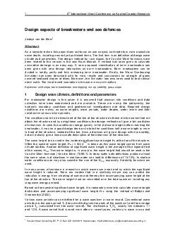
Jentsje van der MeerAs a keynote lecture this paper does not focus on one subject but treats four main aspects to some depth including new not yet published items The first item is on definition of ID: 478690

Jentsje van der MeerAs

Share:

Link:

Embed:

Download Presentation from below link

Download Pdf The PPT/PDF document "International Short Conference on Applie..." is the property of its rightful owner. Permission is granted to download and print the materials on this web site for personal, non-commercial use only, and to display it on your personal computer provided you do not modify the materials and that you retain all copyright notices contained in the materials. By downloading content from our website, you accept the terms of this agreement.


Presentation Transcript

International Short Conference on Applied Coastal Research Jentsje van der MeerAs a keynote lecture this paper does not focus on one subject, but treats four main aspects to some depth, including new not yet published items. The first item is on definition of design wave Van der Meer Consulting BV. P.O. Box 423, 8440 AK, Heerenveen, the Netherlands. jm@vandermeerconsulting.nl SCACR – Proceedings 2011 2 overtopping formulae, is the spectral period T (= m). This period gives more weight to the longer periods in the spectrum than an average period and, independent of the type of spectrum, gives similar wave run-up or overtopping for the same values of T and the same wave heights. In this way, wave run-up and overtopping can be easily determined for double-peaked and "flattened" spectra, without the need for other difficult procedures. It is a wave period that has not been used a lot in breakwater design, yet. For a single peaked spectrum the is close to 1.1. Any formulae can actually be rewritten by the use of this ratio and, in case of bi-modal or flattened spectra, the use of T will then give a more accurate prediction. Wave steepness is defined as the ratio of wave height to wave length, s = H. Here L is the deep water wave length L = 2). With use of T the steepness becomes s, with the mean period T it becomes som and finally, with the period T it becomes ssteepness tells something about the wave’s history and characteristics. Generally a steepness of s = 0.01 indicates a typical swell sea and a steepness of s = 0.04 to 0.06 a typical wind sea. Swell seas will often be associated with long period waves. But also wind seas may become seas with low wave steepness if the waves break on a gentle foreshore. By wave breaking the wave period does not change much, but the wave height decreases. This leads to a lower wave steepness. A low wave steepness on relatively deep water means swell waves, but for depth limited locations it often means broken waves on a (gentle) foreshore. Stability formulae include often the stability number H is the relative buoyant density, = ( - is the mass density of the rock and the mass density of the water. The nominal diameter D = (M is the average mass of the stone class. Actually, D is the "cubical" size of the rock with the average mass, regardless of the actual shape of the rock. Dynamically stable structures like rock, gravel and shingle beaches, can be described by a dynamically stable profile, see Van der Meer (1988-1). Such profiles change with the wave and water level conditions. The wave period has similar effects on the profile as the wave height, meaning that a longer wave period as well as a larger wave height would results in a "longer" profile. It is for this reason that Van der Meer (1988-1) introduced the dimensionless wave height - wave period parameter H, which can be described by: = H (1) With a mean period T the parameter becomes H and with the peak period H. It is this parameter that also has been used in the past, like in PIANC (2003) to describe the recession of berm breakwaters. Dynamically stable structures show some stability for a certain wave condition if a certain profile has been formed and this profile does not change as long as the wave conditions do not change. During every wave action (wave breaking, wave run-up and wave run-down) it is possible that individual stones move up and down, but this does not affect the profile. This is of course not a good situation for a breakwater. Dynamically stable for a berm breakwater means that under severe wave conditions and after reshaping still some stones move up and down the slope during individual wave action. This is different from the movement of rock during reshaping as in that situation rock move to a more stable position and then remain there. Statically stable structures are stable under severe wave attack and only then may show a little movement of rock, called damage. Such damage, S, is related to the eroded area, A, around the water level, see Figure 1. This graph shows the original definition as given in Van der Meer (1988-1) with S as damage and A as erosion area. The definition of damage is: = A (2) Dynamically stable structures can be given by a profile, statically stable structures by the damage S. But what about berm breakwaters? In many cases the berm is not as stable as a statically stable structure and will reshape to some extent. the recession, Rec, of the berm as a parameter to describe the behaviour of berm breakwaters. Figure 2 gives the principle idea of the recession parameter. International Short Conference on Applied Coastal Research Figure 1. Definition of damage for a statically stable structure, Van der Meer (1988-1). Figure 2. Principle idea of recession to describe the behaviour of a berm breakwater. 2 Rock slope stability 2.1 Van der Meer formulae The original Van der Meer formulae for statically stable rock slopes were published in Van der Meer (1988-1), but also in journal papers Van der Meer (1987) and Van der Meer (1988-2). These formulae were also described in the first Rock Manual, 1992. The new Rock Manual, 2007, however, treats a rewritten version of the original Van der Meer formulae, and added the so-called modified Van der Meer formulae for shallow water. It should be noted that these latter formulae were not modified by Van der Meer, but were based on the limited and confidential work of Van Gent et al. (2004). Different from the Rock Manual (2007), only the original Van der Meer formulae will be applied here. The formulae can be applied to shallow water conditions where the significant wave height on the foreshore has reduced to a minimum of 50% of its original value on deep water. The original formulae are given by: For plunging waves: ௡ହ଴ൌ6.2ܲି଴.ହ (3) and for surging waves: ௡ହ଴ൌ1.0ܲ√ܿ݋ݐߙ ߦ (4) The transition of plunging (breaking) waves to surging (non-breaking) waves is given for: ൌൣ6.2ܲ଴.ଷଵ√ݐܽ݊ߙ൧ುశబ.à°± (5) SCACR – Proceedings 2011 4 with: H = significant wave height at the toe of the structure (actually H = relative buoyant density: = ( - = mass density of rock = mass density of water = nominal diameter: D = (M = average mass of the rock class P = notional permeability factor P = 0.1: impermeable core beneath the armour layer P = 0.5: permeable core beneath the armour layer P = 0.6: homogeneous structure (only one rock class) = damage level = number of waves in the considered sea state = breaker parameter: = tan g = acceleration of gravity = mean period from time domain analysis = slope angle Equation 3 applies and for &#x 000; this is Equation 4. For detailed description of the notional permeability factor P, short sea states with N 1000 and long seas states with N&#x 600; 7500, as well as the reliability of the formulae, one is referred to Van der Meer (1988-1, 1988-2, 1987-1) or the Rock Manuals (1992 and 2007). The easiest way to apply the formulae is to use the program Breakwat (commercial software from Deltares) as limitations with respect to the formulae are embedded in this program. The classification of the damage level S for a two-diameter thick rock slope is given in Table 1. The initial damage (some settlement, first rocks moving) is given as S = 2 or 3, depending on the slope angle. Failure of the rock layer is defined as under layer visible. In average about a layer of one diameter thickness will then be removed, with at certain locations a little more, showing the under layer. Intermediate damage is in between initial damage and failure. Table 1 has to be used in designing rock slopes on stability. Table 1: Classification of the damage level SThe original Van der Meer formulae were modified in the Rock Manual (2007), based on the work of Van Gent et al. (2004 - confidential data). They applied a bulk analysis on their data, using the original Van der Meer formulae, but adopting different coefficients. Their work showed less stability in (very) shallow conditions and explanations for this were not given. For very shallow conditions it may well be that the trends in the Van der Meer formulae are no longer valid, like the relationship between damage and storm duration or number of waves, N: ; or the relationship between damage and wave height: . This was not considered in the analysis by Van Gent et al. (2004). The effect in the Rock Manual (2007) is that for rock slopes in shallow water one ends up with a (much) larger rock size than with the original Van der Meer formulae. Another question is to what conditions of "shallow water" the original Van der Meer formulae would be correct. It is true that most of the tests of Van der Meer (1988-1) were performed for relatively deep water. One of the implications is then that the formulae are valid for Rayleigh-distributed wave heights. A limited number of tests in Van der Meer (1988-1) were performed on a 1:30 foreshore with breaking wave conditions. These tests showed that in more shallow conditions the distribution of wave heights is no longer according to a Rayleigh distribution and that less large wave heights occur. It means that in shallow water the stability if the slope initial damage intermediate damage failure (under layer visible) 1:1.5 2 3-5 8 1:2 2 4-6 8 1:3 2 6-9 12 1:4 3 8-12 17 1:6 3 8-12 17 International Short Conference on Applied Coastal Research same significant wave height is present as in deep water. This is logical as less high wave heights are present in the shallow water case. For this reason it has been proposed in Van der Meer (1988-1) to use the H instead of the significant wave height (and adjust the coefficient in the formulae). The important trend in shallow water is that stability increases if waves start to break. Using the H-value in the Van der Meer formulae instead of the H leads for shallow water to a smaller required rock mass. In very shallow water, however, other effects may play a role. If the original significant wave height reduces by breaking to 30% of its original value or even less, the wave steepness becomes very long and the shape of the waves may be very different from less shallow water situations. Short waves or high wave steepnesses do not longer exist for these conditions. It were mainly these kind of conditions that were the subject of the research of Van Gent et al. (2004). In their research, however, they never mentioned that the stability increases for first breaking of waves and they do not distinguish between first breaking and very large breaking. 2.2 Design method for rock slopes The design of a breakwater or rock slope is often concentrated around extreme conditions close to or exceeding the estimated design life of the structure. But that is only a part of the whole picture. The full extreme distribution of wave conditions: wave heights, wave periods and water levels, should be considered. A picture like Figure 3 gives insight in possible wave climates and is a reproduction from PIANC (1992). It shows the (deep water) significant wave height versus the return period, from 1 - 1000 years The curves show the different levels for the 100-years condition, which give an estimation of the severity of the wave climate. Another feature in Figure 3, however, is the steepness of the curves. And this aspect is very important for design of breakwaters or other coastal structures. A flat curve means that wave heights close to a 100-years condition occur fairly frequently, but this condition will never significantly be exceeded. On the other hand, a steep curve means that yearly wave heights may be quite low, but really extreme conditions significantly exceed a 100 years condition. Figure 3. Deep water wave climates (from PIANC (1992)). A good way to consider the whole wave climate for design of a rock slope is to consider a few practical return periods and define associated allowable damage levels. For instance, a small return period should not give any damage, however, for a very extreme return period damage is acceptable, but failure of the slope is not. An example is shown in Table 2, but it should be 1101001000Return period (years) Bilbao Sines Tripoli North Sea Follonica Pozallo SCACR – Proceedings 2011 6 noted that this is an example and could be adjusted according to the client's desire for a more or less conservative structure. Table 2: Example of allowable damage, depending on return period. Return period Allowable damage Rock slopes Concrete units 10 y S = 2 N = 0.2 50-100 y S = 3-5 N = 0.5 300-500 y S = 8-12 N = 1.0 (depending on slope) Equations 3 and 4 (or the program Breakwat) can then be used to calculate the damages or required rock weights for each return period. It depends then on the actual wave climate which condition will be determining for design. In general, for flat curves like the Pozallo curve in Figure 3, the 10-years condition will govern the design. For steep curves, like Bilbao, it will be the very extreme conditions. 2.3 Cumulative damage The Van der Meer formulae are based on one test condition per test. After each test of 3000 waves the slope was reconstructed for the next test. In this way test results were not influenced by earlier test conditions. But in reality a structure will experience many storms with different attitude. Also testing of breakwaters for design is often performed with a series of increasing sea states. The Van der Meer formulae can be applied to such situations by the cumulative damage method, which has been described in Van der Meer (1985-discussion) and which has also been implemented in Breakwat. Figure 4. Cumulative method to calculate damage for various consecutive sea states. In fact the method is fairly easy. A first sea state, given by the significant wave height H, or by , mean period T and number of waves N, gives a calculated damage level S. A second sea state would be defined by H,(or H), T and N. The next calculation is to determine the number of waves Nw12 that is required for the second sea state to create the damage S that was caused by the first sea state. Then the damage S for the second sea state can be calculated, but now by applying Nw12 + N as the number of waves. A third sea state would be calculated by repeating the same procedure. Figure 4 gives an example calculation. The structure has a slope with cot = 1.5, a notional permeability of P = 0.55 and a rock class with average mass M = 10 t and density = 2700 05001000150020002500DamageNumberwaves SeastateHs=4Tm=10Nw=2160 SeastateHs=5Tm=12Nw=1800 SeastateHs=6Tm=14Nw=1543 International Short Conference on Applied Coastal Research kg/m. The mass density of the water is = 1025 kg/m. Three consecutive sea states have been defined. each lasting for six hours: =4 m; T=2160 =5 m; T=1800 =6 m; T=1543 For each of the sea states the S - N curve can be calculated using Equations 3 and 4. The damage development is a straight line for the first 1000 waves and then continues as a square root function . The damage after the first sea state can directly be calculated: = 2.24. This damage is reached for the second sea state for 585 waves. The damage for the second sea state is then calculated for N = 1800 + 585 = 2385 and amounts to S = 5.92. This damage is reached with 738 waves for the third sea state and the final damage is then calculated with N = 1543 + 738 = 2281 and amounts to S = 12.01. The damage for sea state 3 only would be S = 9.96, so the two first seas states increased the final damage by about 20%. 3 Berm breakwaters 3.1 Classification The principle design of reshaping berm breakwaters, as described by Baird and Hall (1984), has been developed further into less reshaping and more stable berm breakwaters with more rock classes compared to only a small and a large class, core and rock. PIANC (2003) gave a classification of berm breakwaters as shown in Table 3. Table 3. Classification of berm breakwaters by PIANC, 2003. Type of breakwater Statically stable non-reshaped. In this condition few stones are allowed to move, similar to the condition for a conventional rubble mound breakwater. Statically stable reshaped. In this condition the profile is allowed to reshape into a profile, which is stable and where the individual stones are also stable. 1.5-2.7 40-70 Dynamically stable reshaped. In this condition the profile is reshaped into a stable profile, but the individual stones may move up and down the front slope. &#x 20-;Ѕ.;瀀2.7&#x 20-;Ѕ.;瀀 70 The classification uses both the stability number H as well as the dimensionless wave height - wave period parameter H. There is a large difference between the parameters as the stability number does not include any wave period effect and the H parameter gives similar effect to wave height and wave period. PIANC (2003) does not conclude on which parameter should be decisive for berm breakwaters, although formulae on recession of the berm have been given as function of HThe classes of statically non-reshaped and reshaped berm breakwaters overlap the range of = 1.5 - 2, although a different range in H is given. This might suggest that a longer wave period results in more reshaping and a less stable profile. Proof of this, however, is not Dynamically stable means that rock will move continuously under (severe) wave attack, which may lead to breaking of the rock and to longshore transport. Significant longshore transport, affecting the stability of the structure, should be avoided at all times. This is different from reshaping, where it is expected that displacement of rock will result in a more stable profile. One may actually conclude that dynamically stable (berm) breakwaters are not acceptable, as breakwaters during their life time should be statically stable. PIANC (2003) has given a classification of berm breakwaters that shows that there are different types of berm breakwaters with different structural behaviour. In that sense the classification in SCACR – Proceedings 2011 8 Table 3 is very useful. But given the remarks above and developing insight in the stability of berm breakwaters, the classification can be updated. The reshaping (mass armoured) berm breakwaterhas a large berm with mainly one rock class. The berm may be long and just above design water level, but may also be quite high - even similar to the crest height - and then with a narrower berm. As the berm will reshape it is mainly the volume or cross-section of the berm that determines the design, not the width of the berm only. The seaward slope of the berm is often quite steep, up to the angle of repose of rock. The structure will be unstable as constructed, but statically stable after reshaping. The behaviour is best described by the profile of the structure and only partly by recession. The construction should be easy without significant requirements and only a few rock classes have to be made, without very large sizes. A reshaping berm breakwater will be stable for overload conditions, but then not much resiliency (reserve capacity) will be left. Experience shows that this kind of berm breakwater may need some maintenance (adding berm rock) during the life time of the structure. A hardly reshaping Icelandic-type berm breakwater will have a high berm and the total cross-section or volume will be less compared to a reshaping berm breakwater. The high berm has also a function as it will absorb the energy of large and long waves overtopping the berm. The hardly-reshaping Icelandic-type of berm breakwaters need fairly large rock, but in small quantities. Getting large rock, using the right experience, shows that this in many cases will not significantly increase the cost of the structure. In many cases the largest class of rock above the water line will be placed according to specifications that enhance stability. In fact these stones can be placed in such a way that rocks on the outer layer are in contact with each other and loose rocks do hardly exist. The mass armoured as well as the Icelandic-type berm breakwater may show only partly recession when designed for it. In this case it is advised to have the berm level of the mass armoured berm breakwater at the same level as the Icelandic-type. The ability to absorb wave energy with a relatively high berm is also good for the partly reshaping mass armoured berm breakwater, as partly reshaping means that quite some part of the berm is left in place. There are, however, no placement specifications for the mass armoured berm breakwater and the seaward slope still may be quite steep. If this is indeed the case, the first reshaping may be earlier than for an Icelandic-type berm breakwater, but after some reshaping they will show similar reshaping or stability. Hardly reshaping berm breakwaters may be described by conventional damage levels S as well as start of recession. For partly reshaping berm breakwaters there will be more damage as well as recession. The fully reshaping berm breakwater only considers recession or actually reshaping. Based on these types of structures a new classification for berm breakwaters, including indicative values for the stability number, the damage and the recession, is shown in Table 4. These values are given for a 100-years wave condition. For wave conditions with smaller return periods the values will be smaller and consequently, for more severe wave conditions, like overload tests, the values may be larger. Table 4. Proposed classification of berm breakwaters. Breakwater H S Rec/DHardly reshaping berm breakwater (Icelandic-type) 1.7 - 2.0 2 - 8 0.5 - 2 Partly reshaping Icelandic-type berm breakwater 2.0 - 2.5 10 - 20 2 - 5 Partly reshaping mass armoured berm breakwater 2.0 - 2.5 10 - 20 2 - 5 Reshaping berm breakwater (mass armoured) 2.5 - 3.0 -- 5 - 12 3.2 PIANC (2003) recession data for berm breakwaters PIANC (2003) presented recession data of many research projects, mainly with traditional reshaping berm breakwaters as well as partly Icelandic-type berm breakwaters, see Figure 5. Most of the data represent a recession larger than 5*D and a stability parameter H larger than 70. A large scatter is present due to various influences. Some of them would be the definition of wave height (at the toe or more at deep water), placement of rock (dumped or carefully placed), way of measuring recession, seaward slope angle, etc. International Short Conference on Applied Coastal Research Figure 5. Recession data from PIANC (2003), including the data in Sigurdarson et al. (2008) on stable Icelandic-type berm breakwaters. As stated above most of the PIANC (2003) data represented large recession and high stability numbers, H. Focusing only on Icelandic-type berm breakwaters changes the area of interest. With the limits of H 70 and not more than 7-8 stones removed across the berm (Rec/D 8) leaves only the data of the lower left corner of Figure 5. In this region there are data points which do not show any recession for H = 40-50 and others that show recession to be 7 or 8 stone wide. Also, there are data points showing recession of 2 stone wide for Hvalues of only 10. The only conclusion is that the data given in PIANC (2003) are not able to give any reliable design guideline for the Icelandic-type berm breakwater. More well-defined data are required to give such guidelines. Sigurdarson et a.l (2008 and 2011) defined requirements for reliable data representing the Icelandic-type berm breakwater and indentified three data sets which fulfilled these requirements: MAST II (1996 and 1997), Myhra (2005) and Sveinbjörnsson (2008). The recession data cover the area shown in Fig. 5 and is really focussed around small recession. They found that the best fit for the recession data was obtained using the parameter Hwhich includes the peak period, T, instead of the mean period, T. But the difference with using only the stability number H = Hn50, so not considering the wave period, was not large. Based on that data Sigurdarson et al. (2008) derived the following formula that provided a reasonable fit to the data shown in Figure 6: Figure 6. Recession data for an Icelandic-type berm breakwater, using the peak period T and showing the recession formula (6) with 90% confidence band as presented by Sigurdarson et al. (2008). 01020304050607080Rec/D Sveinbjornsson h=0.59 m Sveinbjornsson h=0.645 m Sirevag test 2 MAST II test 3 MAST II test 4 Equation 2 90% confidence bands SCACR – Proceedings 2011 10 Rec/Dwith: Rec/D = 0 for H Sc (6) (Sc) = 35 and (Sc) = 5 and H 3.3 New and accurate data set including analysis 3.3.1 Optimized definition of recession A statically stable design of an Icelandic-type berm breakwater has been tested in a wave flume at HR Wallingford, where the behaviour from the start of moving of the first stones, up to a few times an overload condition, was measured very precisely. At the start of damage the recession of the berm profile varies considerably along the profile. But when the damage gets larger and the berm really reshapes into the well-know S-profile, the recession becomes more. In that case it is sufficient to measure only a few profiles, average them and measure the recession, the horizontal retreat of the berm, given in nominal diameter of the armour stone protecting the berm, D. This has often been done in berm breakwater research, also for the less reshaping Icelandic-type berm breakwater. In the research at HR Wallingford a very accurate laser profiler has been used and according to the method in Van der Meer (1988-1) ten profiles have been averaged to give a good description of the behaviour of the structure. Figure 7 shows an example of damage development of the averaged 10 profiles from the pre-test condition, through the full sequence of testing. Some profile or damage development starts, ending in a little reshaping at the end of the test series. Figure 8 shows on the other hand the individual ten profiles after two times the design condition. It is clear that the scatter between the different profiles is considerably larger than the average profile development over the full test sequence. Figure 7. Development of profiles of an Icelandic-type berm breakwater under increasing wave conditions, measured with a laser profiler; each profile is the average of 10 individual profiles. Figure 8. Ten individual profiles of the same Icelandic-type berm breakwater measured with a laser profiler after two times the design event, showing the large scatter of individual profiles. 11 5 International Short Conference on Applied Coastal Research The recession of a berm breakwater is usually defined as shown in Figure 2, that is the horizontal recession on top of the berm. This may be alright for structures that experience considerable recession but not so good for structures experiencing less recession. The damage or displacement of stones usually starts at around the still water level and then proceeds upward. For limited damage, as for the Icelandic-type berm breakwater, the damage might not have proceeded up to the top of the berm where the recession usually is measured. Another practical issue is that the recession on top the berm is not easy to define. The front slope and top of the berm of the Icelandic-type berm breakwater is covered with large stones and when these are profiled, the profile rarely shows a sharp intersection between the front slope and top Therefore, it was necessary to modify the definition of recession to take note of profile development on the full slope from top of the berm down to low water level, not only on top of the berm. The recession is taken as the horizontal difference between the as-built profile of the Class I armour and the profile recorded after the test, see Fig. 9. Two recession parameters have been proposed. The maximum recession distance, Rec, is the greatest recession measured on any individual profile, and the average recession distance, Rec, is the recession of the average profile averaged between low water level and top of the berm. Figure 9. The modified definition of a berm recession. 3.3.2 The dataset The seaward slope of the berm had a slope of 1:1.5. The berm itself is very porous with large rock in the whole berm. According to Van der Meer (1988-1) this would give a notional permeability factor of around P = 0.55 - 0.6. Th can also be found from the profile, which results in the damage parameter S = A. It is, therefore, interesting to make a comparison between damage measured for the Icelandic-type berm breakwater and damage calculated by stability formulae for rock slopes. Details of wave conditions, damage and recession for the three tests are given in Table 5. Design conditions for about 100-years return period are reached for stability numbers of =1.5-1.7. Overload conditions are reached for H = 2.0 - 2.4. Note that in many tests the wave steepness was quite low and therefore the wave period fairly long. This results in fairly large H and H values. Maximum recessions in Tests 1 and 2 amount to about Rec = 5 with damage up to S = 9-12. This is well in the range of rock slope stability, see Van der Meer (1988-1). In Test 2 the rock below swl was placed a little more randomly, resulting in a slightly more damage and recession compared to Test 1. The rock used in Test 3 was slightly larger and more elongated and placed with good interlocking above swl. This resulted in hardy increase in damage and recession for the overload situations. SCACR – Proceedings 2011 12 Table 5. Recession and damage results of 3 tests on Icelandic-type berm breakwater. 3.3.3 Description and comparison of damage Sd The stability formulae of Van der Meer (1988-1) include the significant wave height, mean wave period, slope angle and notional permeability. It is also possible to calculate cumulative damage (mainly through BREAKWAT), which makes it possible to simulate the whole test sequence in a test. In the test sequence (see Table 5) sometimes the wave height was kept the same or even lowered, while the wave period was changed. The stability formulae suggest that stability would increase with increasing wave period, as surging or non-breaking waves are present for a steep slope and with a large notional permeability. Figure 10 shows the measured damage as a function of the stability number. Damage increases as long as the wave height is increased and the increase in damage is small if tests with similar wave heights have been performed. As explained before, only the overload situation in Test 3 (H =2.3) showed remarkable stability, due to specific placement of the larger rock. Figure 10. Damage versus stability number, as measured. Dn50BreakwatTest0.950.01124.628.00.000.201.500.01345.751.01.390.291.670.01253.362.02.810.821.790.03147.143.54.871.541.750.01555.661.15.731.691.990.01566.273.87.182.442.400.03955.060.48.943.92Test0.950.01124.828.20.000.290.081.490.01345.450.72.450.860.841.680.01248.963.65.132.102.331.650.01943.648.85.802.312.961.690.01351.262.56.262.553.541.940.01464.571.99.154.104.902.360.03853.959.211.565.207.161.660.01452.958.111.625.197.16Test0.880.01022.525.80.000.150.051.380.01241.546.40.710.250.541.500.01345.052.01.370.201.071.560.01344.954.91.560.361.711.710.03144.240.41.900.502.611.600.01350.156.12.310.512.641.540.01346.054.22.010.562.641.850.01460.568.32.400.563.672.300.03751.958.02.431.215.86 00.511.522.53DamageStabilitynumbern50 test test test 13 5 International Short Conference on Applied Coastal Research Figure 11. Damage versus stability number, measured and calculated. For Test 2 Figure 10 shows a similar damage of S =2.36 and 1.66. Actually, in the last test the wave height was lowered (and the wave period increased), but this did not lead to larger damage. Figure 11 is similar to Figure 10, but now the results of the damage calculations have been included. The cumulative damage was calculated for Test 2 (open squares), which has actually similar conditions as Test 1, and also for Test 3 with different rock size and test conditions (open triangles). Results of calculations depend on the input. The original Van der Meer equations were used through Breakwat and cumulative damage was calculated. The berm is very permeable, but the structure is not completely a homogeneous structure. For this reason a notional permeability factor of P = 0.55 was used. The seaward slope of the berm breakwater is 1:1.5. But it would not give a correct comparison if this slope was used in the calculations. The berm breakwater has a horizontal berm and also some horizontal parts below water level (between rock classes I and II and at the toe). The average slope from toe to the crest level was close to 1:2 and therefore this slope angle was used for calculations. Calculated damages are slightly lower for Test 3 than for Tests 1 and 2, which is according to the measurements. It is clear, however, that the berm breakwater in Test 3 showed very good behaviour for the final wave height, better than the prediction of the stability formulae. Note also that the calculations give similar damage for the last two test series in Test 2, where the wave height was lowered (with an increase in wave period). This is completely according to the measurements, although the damage in average was a little larger in the tests than predicted by the stability formulae. It can be concluded that the stability formulae for rock slopes in average give a fairly good prediction of the damage at the seaward side of a statically stable Icelandic-type of berm breakwater. The measurements also confirm the stability formulae in the sense that a larger wave period does not really increase damage. Wave height seems to be more important than wave period. 3.4 Detailed analysis of recession Rec Figures 12 and 13 show the development of the average recession, as defined in Figure 9, for the three tests. In Figure 12 the recession is given versus H, which is comparable with Figure 6. Figure 13 uses H instead of H, and is more comparable with Figure 10. The data points have been connected by lines as this shows better the sequence of the test series in the test. Figure 12 clearly shows where sometimes the H condition was lowered (similar or even larger wave height, but with smaller wave period). If the use of H would be correct, then a significantly lower H value should lead to significant increase of recession. All tests, however, show that recession increases, even with a much lower H 00.511.522.53DamageStabilitynumberDn50 test test test Breakwattest Breakwattest SCACR – Proceedings 2011 14 Figure 12. Average recession Rec versus HThat is different in Figure 13, where damage increases if H increases and where damage remains the same if the wave height is reduced. Figure 13 shows a similar behaviour as for the damage in Figure 10. Again it must be concluded that the wave period has hardly any effect on recession and that the wave height is the governing parameter. Figure 13. Average recession Rec versus Hs/It does not mean that the parameter H is not a good parameter to describe recession or reshaping. The parameter was developed for dynamically stable structures like gravel and cobble beaches, see Van der Meer (1988-1), and also performs well for really reshaping berm breakwaters with H around 3. But start of damage or recession describes more statically stable rock slopes (specifically almost homogeneous structures) and here stability and recession are not really influenced by the wave period. Figure 6, taken from Sigurdarson et al. (2008), shows three data sets with Equation 6 as prediction formula. Figure 14 shows the same data, but now with the data of the new tests. As in many test series long wave periods were applied, most of the tests are on the right side of the prediction curve and far outside the 90% confidence band. As concluded above, it is not a good way to include the wave period for start of recession, comparable to statically stable rock slopes. Figure 15 shows the average recession versus the stability number Hn50Test 2 fall exactly within the earlier data, Test 1 shows a little more reshaping and Test 3, for the final wave height, a little lower. The points of Sveinbjornsson (2008) with Rec = 0 are mainly due to inaccuracy as only one profile was measured, not ten as in the latest tests. 01020304050607080AveragerecessionRecn50 Reav/Dn50test Reav/Dn50test Reav/Dn50test 0.00.51.01.52.02.53.000.511.522.53AveragerecessionRecn50StabilitynumberDn50 Reav/Dn50test Reav/Dn50test Reav/Dn50test 15 5 International Short Conference on Applied Coastal Research Figure 14. Average recession versus H and data of Sigurdarson et al. (2008). Figure 15. Average recession Rec versus H, with data from Sigurdarson et al. (2008) and with a new prediction formula. A formula that fits closely to the majority of the data points in Figure 15 is given by: Rec = 3.5 (H (7) with: Rec = 0 for H c (Sc) = 1.3 and (Sc) = 0.2 and Hn50The formula shows that for a statically stable Icelandic-type berm breakwater with a design value of H = 1.5 the expected recession is not more than about half a stone diameter. = 2.0 this may increase to 1.5 to 3 stone diameters, depending on how accurate the rock above swl has been placed. 01020304050607080Rec/Dn50 Sveinbjornsson (2008) Myhra (2005) MAST II (1996) Eq. 2008 New test 1 New test 2 New test 3 0.00.51.01.52.02.53.0Rec/Dn50Dn50 Sveinbjornsson (2008) Myhra (2005) MAST II (1996) New test 1 New test 2 New test 3 Recession equation 90% conf. band SCACR – Proceedings 2011 16 4 Wave overtopping and run-up simulactive tests at grassed slope of dikes and boulevards 4.1 The Wave Overtopping Simulator The Wave Overtopping Simulator was developed in 2006 and destructive tests have been performed in February and March of 2007 - 2011 and in November and December 2010. The tests show the behaviour of various landward slopes of dikes, embankments or levees under simulation of wave overtopping, up to a mean overtopping discharge of 125 l/s per m. All research performed was commissioned by the Dutch Rijkswaterstaat, Centre for Water Management. The research was performed by a consortium of partners and was led by Deltares. Consortium partners were Deltares (project leader, geotechnical issues, model descriptions, hydraulic measurements), Infram (logistic operation of testing), Alterra (grass issues), Royal Haskoning (consulting) and Van der Meer Consulting (performance of Wave Overtopping Simulator and hydraulic measurements). The process of wave overtopping on a dike, levee, seawall or embankment is well known, see the Overtopping Manual (2007). In contrast, the erosive impact of wave overtopping on these structures is not known well, mainly due to the fact that research on this topic cannot be performed on a small scale, as it is practically impossible to scale clay and grass down properly. Only some tests have been performed in large wave flumes, like the Delta flume in the Netherlands and the GWK in Germany, see Smith (1994) and Oumeraci et al. (2000). But these tests are costly and the dike can only partly be modelled. Therefore, the Wave Overtopping Simulator has been developed, see Van der Meer et al. (2006, 2007 and 2008) for more details. The Simulator consists of a high-level mobile box to store water. The maximum capacity is per m width (22 m for a 4 m wide Simulator). This box is continuously filled with a predefined discharge and emptied at specific times through a butter-fly valve and a guidance to the crest, in such a way that it simulates the overtopping tongue of a wave at the crest and inner slope of a dike. The discharge of water is released in such a way that for each overtopping volume of water the flow velocity and thickness of the water tongue at the crest corresponds with the characteristics that can be expected. See Figure 16 for the principle of the Wave Overtopping Simulator. Various overtopping volumes are released randomly in time, see Figure Figure 16. Principle of Wave Overtopping Simulator. Field tests on real dikes have been carried out from 2007 - 2011, all at the end of the winter and one in November/December, when grass roots are in worst condition. Figure 18 shows the set- 17 5 International Short Conference on Applied Coastal Research up of the simulator at the crest and seaward side of a dike and very close to a highway. The design and calibration of the Wave Overtopping Simulator has been described by Van der Meer (2007) and the test results of the first tested dike have been described by Akkerman et al. (2007-1 and 2007-2). Part of the tests in 2008 have been described by Steendam et al. (2008). A summary report on all the testing in 2007 and 2008 has been described by Van der Meer (2008). Tests and results of 2009 - 2010 have been described in Steendam et al. (2010, 2011) and Van der Meer et al. (2009, 2010, 2011). Figure 17. Release of a wave. Figure 18. Set-up of Wave Overtopping Simulator close to a highway (February 2009). Most test conditions were given by a mean discharge and lasted for 6 hours. Test conditions increased from 0,1 l/s per m to 1; 10; 30; 50 and 75 l/s per m. A full test on a dike section took about one week and often more than 14,000,000 litres of water flowed over the inner slope of 4 m width. Each test condition consisted of simulation of the required distribution of overtopping volumes (see the Overtopping Manual (2007)). Such a distribution depends on expected conditions at sea: a larger significant wave height (as at sea dikes) will show fewer overtopping waves, but the volume in the overtopping waves will be bigger than for a smaller wave height (as for example at river dikes). All tests until now have assumed a significant wave height of 1, 2 or 3 m with a wave steepness of 0.04 (using the peak period). Distributions of overtopping volumes for a condition with 2 m wave height and for various mean discharges are given in Figure 19. Figure 19 clearly shows that for each mean discharge there are only a small number of waves that give large overtopping volumes. The general behaviour of wave overtopping can be described by a large number of fairly small overtopping waves and a few which are much bigger. These few but bigger waves often cause the damage to the inner slope. SCACR – Proceedings 2011 18 In the first years of testing it appeared to be very difficult to measure any hydraulic parameter on the inner slope, like flow velocity or flow depth. The velocities can approach 8 m/s and the water is very turbulent with a lot of air entrainment, see also Figure 17. Laboratory instruments have not been designed for this kind of conditions. In 2009 a lot of attention was focussed on improving the measurements. Amongst them a floating device to measure the flow depth and front velocities of an overtopping wave. The floating device is a curved board which has been hinged about 1 m above the slope and which floats on top of the flowing water. The rotation at the hinge is measured and gives the flow depth. Figure 20 shows the record of this floating device for three consecutive overtopping volumes of 3.0 m per m width each. Recording started exactly when the signal was given to open the valve. The overtopping volumes and the records of flow depth reproduce very nicely. The maximum flow depth was about 0.25 m. Figure 19. Distribution of overtopping volumes of waves for sea dikes and various mean overtopping discharges, as simulated by the Wave Overtopping Simulator. Figure 20. Record of flow depth with floating device for 3 overtopping waves of 3 m/m. 4.2 Destructive field tests 4.2.1 Failure mechanisms Wave overtopping may lead to failure of the crest and landward slope of a dike. In principle there are two different failure mechanisms. Fast overtopping water may damage the surface of the crest and landward slope and, if initial damage or erosion has occurred, this may continue to the layer underneath the grass cover and may lead to an initial breach. This is actually the process which is simulated by the Wave Overtopping Simulator: erosion of the slope. A major failure mechanism on steep landward faces (typically 1:1.5 and 1:2) in the past was slip failure of the landward slope. Such slip failures may lead directly to a breach. For this reason most dike designs in the Netherlands in the past fifty years have used a 1:3 landward slope, where it is unlikely that slip failures will occur due to overtopping. This mechanism might however occur for landward slopes steeper than 1:3 and should then be taken into account in 19 5 International Short Conference on Applied Coastal Research safety analysis. This failure mechanism is NOT simulated by the overtopping tests, as a slip failure needs more width to develop than the 4 m wide test section. Another test method should be used to investigate this failure mechanism, which is not described in this paper. 4.2.2 Locations of tests In total eight locations, seven in the Netherlands and one in Belgium were tested on wave overtopping, see Figure 21. Various tests were performed at each location, in total 27 tests on grassed or reinforced slopes, with or without objects like trees and stair cases. Figure 21. Locations of testing in the Netherlands and Belgium. 4.2.3 Some observations The easiest way to describe observations of the testing is by photographs. This section gives an some examples of observed damages for each tested location. Each photograph has a legend describing the observation. For a complete overall view one is referred to the given references Figure 22. Final result Delfzijl, Groningen, sections 1 and 2. No damage after 50 l/s per m. Left: test section 1 of the present dike after manual initiation of damage (four holes in the slope: 1x1x0.05 m; 0.4x0.4x0.15 m; in the upper part two holes 0.15x0.15x0.15 m) and after 6 hours with 50 l/s per m. Gulley development for the two largest holes, none for the smaller. Right: a reinforced section 2 with geotextile, again after manual initiation of damage, where no gulleys were developed. DelfzijlBoonwegSt PhilipslandKattendijke AfsluitdijkVecht Tholen Antwerp SCACR – Proceedings 2011 20 Figure 23. Delfzijl, Groningen, section 3. Bare clay (0.2 m grass cover was removed). Mean discharges of 1; 5; and 10 l/s per m, each during 6 hours. Ongoing erosion during each condition, which resulted in head cut erosion: a horizontal part with a vertical slope; the vertical slope erodes by lumps of clay from the vertical front and the hole increases upwards. Figure 24. Final result Boonweg, Friesland, sections 1 and 2. No damage after 75 l/s per m. In the last hour of 75 l/s per m damage to the toe (hidden path of brick stone, see photo right). Figure 25. Final result Boonweg, Friesland; section 4. After 5 hours and 51 minutes with 75 l/s per m. The sand core has been eroded to at least 1 m depth and the right side wall is about to collapse. Final result about 45 minutes after first damage was observed. 21 5 International Short Conference on Applied Coastal Research Figure 26. Final result St Philipsland, Zeeland. Damage to the rear side at the maintenance road, which started at 30 l/s per m. Removal of the whole maintenance road. Picture taken half way the 75 l/s per m test. The hole became at the end 15 m wide and about 1 m deep. Figure 27. Kattendijke, Zeeland, section 1. Damage to the rear side at the maintenance road, which started at 30 l/s per m. Removal of the whole maintenance road. Picture taken half way the 75 l/s per m test. The hole became at the end 15 m wide and about 1 m deep. Figure 28. Afsluitdijk. Grass toe, section 1. Grass ripped off on many locations on the slope and completely at the horizontal part, where a section of 4x4 m2 was created without grass. The good clay (still with roots) showed hardly any erosion and resisted without problems 75 l/s per m. Erosion holes near toe about 0.4 m deep. SCACR – Proceedings 2011 22 Figure 29. Afsluitdijk. Staircase with fence, before and after testing, section 3. Left: before testing and right: after 2 hours of 75 l/s per m. The concrete staircase is near failure. Grass ripped off the slope, but gulley development occurred only along the staircase where concentration of flow was observed. Hardly damage to the clay layer. The brick path to the staircase was completely destroyed, as well as the fence gate. Two erosion holes developed at the toe, due to the concentrated flow along the staircase. Holes about 1 m deep, but not reaching the sand core (cover by 0.4 m clay and 1 m boulder clay). Situation after 2 hours of 75 l/s per m. A tested landward slope of a dike, covered with a good grass cover on clay, never failed by erosion due to overtopping for a mean overtopping discharge of 30 l/s per m or less. Only one section failed at 50 l/s per m; some at 75 l/s per m, but part of the sections did not fail, even not for 75 l/s per m. More recent tests at Tholen and near Antwerp with a very bad grass cover, however, showed early failure, even up to 1 l/s per m. The grass cover is very essential for the strength of the slope. It seems that the large erosion resistance of the landward slope of a dike is determined by the combination of good grass cover and clay. The grass cover or mattress seems stronger if it grows on a sandy clay. Such a grass cover may resist even up to 75 l/s per m, but if significant damage occurs, the clay layer is not very erosion resistant (Figure 25). On the other hand, a 23 5 International Short Conference on Applied Coastal Research good quality clay does not produce a very strong grass cover (it is difficult for roots to penetrate into the clay) and the grass may rip off for overtopping discharges around 30 l/s per m (Figure large erosion resistance against overtopping waves. This leads to the conclusion that a good grass cover on a sandy clay and a worse grass cover on good clay show different failure mechanisms, but they show more or less similar strength against wave overtopping. The variability of the grass sod may, therefore, have less influence on the total strength than previously anticipated, except that there should be a fairly well closed grassed cover layer. This could lead to the conclusion that the way of maintenance of the grass has only minor effect on the strength of the landward slope as long as closed grass cover is present. The test at St Philipsland may show that the bad grass (small open areas without grass) on sandy clay may show less resistance (Figure 26). Transitions from slope to horizontal are probably the most critical loincreasing damage (Figures 24, 26 - 28). During the tests this was often the transition from the landward slope to the toe of the dike, with or without a maintenance road. The tests in 2009 were focused on these kind of transitions. Damage was initiated by a mean discharge of 10 l/s per m or more. As the damage occurred at the lowest part of the landward slope it will take time for damage to extend to the crest level and subsequently cause a dike breach. Transitions higher on the landward slope (cycle paths, stability or piping berms with or without maintenance road, tracks of tractors, roads crossing the dike), which have not yet been investigated, might be more critical. Further investigation may give more confirmative conclusions. A hole in the layer of clay, which reaches the under laying sand core and created at a large mean overtopping discharge of 50 l/s per m or more, will give a very quick ongoing erosion. This has not been observed for smaller overtopping discharges, for the simple reason that these smaller discharges never created significant damage to the landward slope. But a test on a parking place of bricks showed that sand erosion with 30 l/s per m, and even with 10 l/s per m, goes fairly quickly. It must be noted that although the test was stopped for 30 l/s per m due to fast ongoing damage to the parking area, the dike itself was not in danger at all. Small obstacles like poles did not show any erosion. Small holes from mice and moles did not initiate damage to the grass cover layer. Also a fence and a little bigger pole (0.15 m by 0.15 m) showed no initiation of erosion. The grass around a fence at the toe of the dike had some influence on initiation of erosion, probably due to larger forces in this area. An obstacle like a concrete staircase on the landward slope was totally destroyed at a stage with 75 l/s per m overtopping (Figure 29). It should be noted, however, that also here the dike itself was not in danger, due to the large erosion resistance of the clay. Still, further research may give more final conclusions on other large obstacles. 4.3 Erosional indices The first three years of testing in the Netherlands with the Wave Overtopping Simulator was done for an assumed wave condition of H = 2 m and T = 5.7 s, being an average wave condition for the Dutch dikes. But estuaries, rivers and small lakes may have design conditions which are smaller, whereas dikes directly facing the North Sea may have larger conditions. It is the crest freeboard that governs the actual overtopping discharge, but the wave conditions determine how overtopping occurs. Larger waves give larger overtopping volumes, but less overtopping waves. From that point of view the overtopping discharge does not describe the full story of wave overtopping. The objective of tests with the Wave Overtopping Simulator is to test the erosional strength of the crest and landward slope against wave overtopping. But do different wave conditions indeed give different moments for damage or failure of the grass? Tests performed in February and March 2010 at the Vechtdijk near Zwolle were performed with different wave conditions, in order to establish the influence of wave climate on erosional resistance. The tests have been described by Steendam et al. (2010). The wave conditions are given in Table 6 and can be characterized by wave heights of 1 m, 2 m and 3 m. A wave height of 1 m gives almost two times more incident waves in 6 hours than a wave height of 3 m. SCACR – Proceedings 2011 24 Table 6. Wave conditions simulated at the Vechtdijk, Zwolle. Seaward slope 1:4 Test duration 6 hours Wave height H 1 m 2 m 3 m (s) 4.0 5.7 6.9 Mean period T (s) 3.3 4.7 5.8 Number of waves N6545 4596 3724 Run-up, Ru (m) 1.99 3.98 5.94 The three wave conditions give different overtopping parameters, like the crest freeboard, percentage of overtopping waves, number of overtopping waves and largest overtopping wave volume, all related to a certain overtopping discharge. All these values have been given in Table 7. A wave height of 1 m, for example, gives for an overtopping discharge of 10 l/s per m 2336 overtopping waves in 6 hours. For a 3 m wave height this reduces to 456 overtopping waves, which is only 20% of the number for 1 m waves, but the overtopping discharge is the same. It is clear that the larger wave height will then give larger overtopping volumes, which in this example is 4.5 m/m as largest volume for a 3 m wave height and only 1.2 m/m for a 1 m wave height. Table 7. Wave overtopping for three wave heights. Mean overtopping discharge q (l/s per m) 0.1 1 5 10 30 50 Crest freeboard R (m) 2.24 1.63 1.2 1.02 0.73 0.6 Percentage overtopping waves P0.7 7.2 24 35.7 59 70 Number overtopping waves N45 471 1573 2336 3861 4583 Maximum overtopping volume V 256 440 831 1197 2359 3401 Crest freeboard R (m) 5.06 3.84 2.98 2.61 2.03 1.76 Percentage overtopping waves P0.2 2.7 11.4 18.9 36.6 47 Number overtopping waves N9 126 525 867 1683 2160 Maximum overtopping volume V 769 1222 2018 2697 4707 6387 Crest freeboard R (m) 7.98 6.16 4.89 4.35 3.48 3.08 Percentage overtopping waves P0.085 1.49 7.05 12.3 26.1 34.9 Number overtopping waves N3 55 262 456 972 1300 Maximum overtopping volume V 1424 2254 3478 4509 7375 9709 The Vechtdijk was a 100% sandy dike, strengthened with only a good grass cover. It was expected that failure of the grass would certainly be achieved for each of the wave conditions and probably for different overtopping discharges. This was, however, not always the case due to early failure of a tree in the slope and a particular transition (see Steendam et al. (2010)) and it was not always possible to reach failure of the grassed slope itself. It became also clear that it is not so easy to decide when a grassed slope has start of damage, developing damage or failure. Failure is the most easy definition: the sand core underneath the soil layer becomes free and damage develops fast. Start of damage would actually be the first small hole in the grass cover and this is not a consistent parameter as it may depend on the existence or non-existence of one weak spot on a fairly large surface. A more consistent definition would be "various damaged locations", meaning that it does not depend solely on one 25 5 International Short Conference on Applied Coastal Research weak spot. In the case the grassed slope did not fail the condition "no failure" became also a criterion. In summary the following damage criteria were used: First damage (Figure 30); Various damaged locations (Figure 31); Failure (Figure 32); Non-failure after testing (Figure 33). Figure 30. First damage. Figure 31. Various damaged locations. Figure 32. Failure. Figure 33. Non-failure after testing. The theory of shear stress with a threshold was taken as a basis for development, see also Hoffmans et al. (2008). The development, however, took place at the same time when Dean et al. (2010) worked on their erosional equivalence, but it was not yet published at that time. Dean et al. (2010) considered three possible developments, which in essence can be described as follows: Erosion due to excess velocity: E = K ) t) [m/s] (8) Erosion due to excess shear stress: E = K ) t) [m/s] (9) Erosion due to excess of work: E = K ) t) [m/s] (10) In all cases the velocity of the overtopping wave plays a role and a critical velocity, which should be exceeded before erosion will take place. In the equations also the time that the critical velocity is exceeded, is important. SCACR – Proceedings 2011 26 The analysis of the Vechtdijk results had as basis Equation 9 (Hoffmans et al. (2008)). The testing showed indeed that only waves of a certain volume (or velocity) damaged the slope. Smaller volumes did not contribute to the development of damage. This confirms the use of a threshold like u. But one main modification was made, based on observed behaviour during testing. In Equations 8 - 10 the time that u is exceeded is taken into account. The origin of this comes from tests with continuous overflow, where indeed time, or the duration that the flow is present, is important. But (severe) wave overtopping is different from continuous overflow. First of all, velocities in an overtopping wave are much larger than velocities in continuous overflow, for the same discharge. Secondly, the duration that u is exceeded in an overtopping wave is quite short, in the order of 1-3 s, and this duration is fairly constant and in total much shorter than for continuous overflow. The observation of overtopping waves has taught us that a wave front rushes over the slope with large velocity. Within tenths of seconds (see Figure 20) the maximum velocity is reached. The grass feels this as a kind of "impact" and it is this impact that causes initiation or further development of damage. It is believed that this impact is more important than the duration of the overtopping wave above a certain threshold. For this reason Equation 9 was rewritten to an erosional index called "cumulative overload", where the actual time or duration for an overtopping wave was omitted: Cumulative overload: ) [m] (11) With known distributions of overtopping wave volumes and known velocities per overtopping wave volume it is possible to calculate the cumulative overload for each wave overtopping condition, or a number of tests, to a certain moment when a damage criterion is reached. And the cumulative overload depends of course on the critical velocity u that is taken. The main question is then: what is the critical velocity, u, that brings the damage observed for different hydraulic regimes, together? The four damage criteria, see Figures 30-33, were taken for all tests and the results were compared for critical velocities of 0; 3.1; 4.0; 5.0 and 6.3 m/s, which are in accordance with overtopping wave volumes of 0; 0.25; 0.5; 1 and 2 mThe following conclusions could be made for the Vechtdijk: A critical velocity should be used of u = 4 m/s (V Start of damage: ) = 500 m Various damaged locations: ) = 1000 m Failure (by mole holes): ) = 3500 m Non-failure for normal slope: ) 6000 mA confirmation of above analysis and conclusions could be established by looking at the damage on the slope after hydraulic measurements. Here only about 40 overtopping waves rushed down the slope instead of many hours like for normal testing, but many large volumes were present. The hypothesis of cumulative overload should work for many hours of testing, but also for the "artificial" distribution of a small number, but mainly very large overtopping waves. The observation of the slope after the hydraulic measurements could best be described as "various damaged locations". A number of small holes were observed and one location with a little larger damaged area. The cumulative overload for these 40 waves, using u = 4 m/s, amounted to 946 m. This is very well comparable with the 1000 m that was given for this damage criterion. It can be concluded that this very short session of large waves can very well be compared with many hours of testing of real wave overtopping. The analysis confirmed the hypothesis of cumulative overload. 27 5 International Short Conference on Applied Coastal Research In future also the method of "excess of work" (Equation 10), which was preferred by Dean et al. (2010), should be elaborated, maybe with ongoing work in the US with a new Wave Overtopping Simulator (see Van der Meer et al. (2011) and Thornton et al. (2011). The reason for Dean et al., however, to choose for excess of work instead of excess of shear stress was that excess of work fitted better to known stability curves for continuous overflow, not wave overtopping. Dean et al. (2010) did not possess the results of simulation of wave overtopping at real dikes as in the Netherlands. Another difference between the two methods is the value of the critical velocity ucontinuous overflow critical velocities are in the range of 1-2 m/s. But the very "weak" Vechtdijk (sand with a good grass cover) needs a critical velocity of 4 m/s and this can be considered as a lower boundary. Other dike sections tested need probably a critical velocity in the range of 5-7 m/s. It is, therefore, still an open question which method would work best with real wave overtopping at dikes. 4.4 Forces on vertical walls The Belgium Integrated Master Plan for Coastal Safety has been developed to protect the coast sufficiently against severe storm events. Weak spots have been determined, and safety measures were proposed, based on an intense campaign of numerical and experimental research. One of these measures are storm walls located at 10 to 15 m behind the crest of a dike or boulevard (along the coastline) or quay wall (in harbours). These walls are designed to withstand wave impacts and are therefore subject to very high forces. The magnitude of these forces and force-over-time signal will determine the foundation, rebar and dimensions of the walls. But also a lot of buildings exist on top of the sea wall and overtopping waves could hit walls of such buildings. Figure 34. Impression of wave force measurements. Up till now, there are no theoretical formulae which allow design engineers to estimate these wave forces on a storm wall due to overtopping waves. The Wave Overtopping Simulator was therefore used to simulate an overtopping wave which impacts a storm wall located at 10 m behind the crest (Figure 34). Two aluminium plates acted as storm walls: one vertical (1.7 m high x 0.5 m wide) and one horizontal (0.5 m high x 1.7 m wide). Each plate was equipped with 4 force sensors, one in every corner of the plate. The force records of the 4 sensors in the vertical plate are shown in Figure 35. SCACR – Proceedings 2011 28 Figure 35. Force record over time on a vertical plate, for a wave of 3500 l/m. The force record of a bottom sensors (red/blue - upper records) shows a very steep rise over time, and reach much higher values than the top sensors (purple/green - lowest records). The flow depth, located near the bottom sensor, is a governing parameter for the force distribution over height. In Figure 36 the maximum forces per meter width on the horizontal plate (0.5 m high) and the vertical plate (1.7 m high) have been plotted versus the overtopping wave volume. There is a very clear trend between both Horizontal plate: F = 2.24 V (11) Vertical plate: F = 0.13V + 2.22V (12) with: F = force per meter width (KN/m) V = overtopping wave volume (m Figure 36. Force as a function of volume. Horizontal plate blue, vertical red. The difference between horizontal and vertical plate is rather small, despite the vertical plate being 3 times higher. The flow depth is a governing parameter for the force distribution over As first analysis it can be concluded that: the wave forces rise very fast, but no impulse peak is visible; wave forces on a wall oriented 45 degrees to the wave direction result in a force that is a factor 2 smaller than perpendicular wave attack; the wave force above the flow depth is negligible. 29 5 International Short Conference on Applied Coastal Research 4.5 Wave run-up simulation The idea of the Wave Run-up Simulator is based on the experiences with the Wave Overtopping Simulator, see the previous sections. It is possible to simulate wave tongues overtopping a dike crest in reality. It must also be possible to simulate waves in the run-up and run-down zone of the seaward slope. This is the zone after waves have broken and when they rush-up the slope. This section describes shortly this new idea of the Wave Run-up Simulator, why it is useful to develop the machine, to perform research with it and to develop a prediction method for slope strength. In fact, a prediction method can already be developed from the Cumulative Overload Method, which was developed on the basis of results with the Wave Overtopping Simulator, see Section 4.3. It also means that tests on the seaward slope will be done for validation purposes only. Not a lot of research has been performed to describe the wave run-up process in detail, physically nor statistically. The first question is whether it is useful to develop and construct a Wave Run-up Simulator to look at strength of seaward slopes with grass coverage. The majority of Dutch seadikes, however, have a run-up zone at the seaward side, above a protected berm at storm surge level, which is covered with grass. Right now no validated safety assessment method exists for these kind of slopes above the wave impact zone. Flow velocities, run-up levels and flow depths must be known over the full run-up zone in order to make a good simulation. Some research has been performed, but never with the objective to design a Wave Run-up Simulator. For this reason a detailed analysis has been performed on what is known in literature and on analysis of existing data from tests. One method is to look at the records of wave run-up gauges. The derivative of the location of the up-rushing wave front gives the front velocity over the full run-up zone, not only at a fixed position. It appears that the velocity along the slope does not linearly decrease with the run-up level. Almost from the start of run-up to about three quarters of the maximum run-up level the flow velocity is high and close to the maximum velocity. The velocity decreases suddenly in the last quarter of the run-up. This conclusion returns in the final description of flow velocities in the run-up zone, see Fig. 37. An average trend exists that flow velocity increases with increasing maximum run-up level, but a large range of flow velocities exist for similar run-up levels. This is more or less similar to waves: various wave periods exist for similar individual wave heights. Wave height as well as wave periods have both a certain distribution and are not directly correlated by an equation. The simulation of up-rushing waves in the run-up zone must exist of the simulation of different flow velocities, whilst a similar maximum run-up has to be reached. This can only be realized if the opening of the valve of the Simulator is part of the steering for the run-up. This method has already been developed for the Wave Overtopping Simulator in the US (Van der Meer et al., 2011). Figure 37. Relative maximum velocity versus relative run-up on the slope. SCACR – Proceedings 2011 30 The maximum velocity on a slope during an individual wave run-up can be calculated by: (13) as stochastic variable with ) = 1.0 and a normal distribution with V = 0.25. A first pilot test with the actual Wave Overtopping Simulator has been performed in March 2011, without any modifications to the Simulator. The Simulator was placed on the seaward slope and berm at storm surge level (asphalt) and run-up simulation started at this almost horizontal berm. The upper grass slope had a 1:3 slope and the Simulator was able to create run-up as well as wave overtopping at the dike crest, see Fig. 38. The maximum run-up was 3.5 m (measured vertically). After up-rush the water comes back in the run-down and in order to release this water the Simulator was placed 0.2 m above the slope. Measurements were performed on up-rush as well as down-rush, on velocities and flow depths. Five test conditions were conducted, starting with a low 2%-run-up level. This run-up level was increased with each following test. Damage was developed at the transition from berm to upper slope, see Fig. 39. The theoretical and practical test procedure will be described elsewhere. Figure 38. Pilot test on wave run-up simulation Figure 39. Damage after 5 tests with various Ru -levels 31 5 International Short Conference on Applied Coastal Research 5 Acknowledgments Although a keynote lecture is given by one person only, the work described in this paper has become available through cooperation with many colleagues from various companies, universities or institutes. Acknowledged is Sigurdur Sigurdarson of IceBreak Consulting Engineers for his excellent cooperation on berm breakwaters. Furthermore, the SBW-project group on "Strength of grass covered dikes due to wave overtopping" is acknowledged for many years of cooperation: André van Hoven (Deltares), Henk Verheij (Deltares), Gijs Hoffmans (Deltares), Gosse Jan Steendam (Infram), Maurice Paulissen (Alterra) and Gert-Jan Akkerman (Royal Haskoning). Akkerman, G.J., P. Bernardini, J.W. van der Meer, H. Verheij and A. van Hoven, (2007-1). Field tests on sea defences subject to wave overtopping. Proc. of Coastal Structures Conference. Venice. Akkerman, G.J, K.A.J. van Gerven, H.A. Schaap and J.W. van der Meer, (2007-2): Wave overtopping erosion tests at Groningen sea dyke. ComCoast, Workpackage 3: Development of Alternative Overtopping-Resistant Sea Defences, phase 3. See www.comcoast.org. Baird, W.F. and K.R. Hall, (1984): The design of breakwaters using quarried stones. ASCE, Proc. ICCE, Houston, 2580-2591. Battjes, J.A. and H.W. Groenendijk, (2000): Wave height distributions on shallow foreshores. Journal of Coastal Engineering 40 (2000) 161-182. Dean, R.G., J.D. Rosati, T.L. Walton and B.L. Edge, (2010): Erosional equivalences of levees: Steady and intermittent wave overtopping. Journal of Ocean Engineering 37 (2010) 104-113. EurOtop Manual, (2007). Wave Overtopping of Sea Defences and Related Structures – Assessment Manual. UK: N.W.H. Allsop, T. Pullen, T. Bruce. NL: J.W. van der Meer. DE: H. Schüttrumpf, A. Kortenhaus. www.overtopping-manual.com. Hoffmans, G., G.J. Akkerman, H. Verheij, A. van Hoven and J.W. van der Meer, (2008): The erodibility of grassed inner dike slopes against wave overtopping. ASCE, Proc. ICCE 2008, Hamburg, p. 3224-3236. MAST II, (1996): Influence of Permeability and Stone Gradation. MAST II – Berm breakwater structures. Contract MAS2-CT94-0087. Myhra, H., (2005): Berm breakwaters. Influence of construction method and storm duration on stability. Ice ride-up. MSc-thesis NTNU, Norway. Oumeraci, H., H. Schüttrumpf, J. Möller and M. Kudella, (2000): Large scale model tests on wave overtopping with natural sea states. LWI-Bericht Nr. 852. Overtopping Manual, (2007). EurOtop. Wave Overtopping of Sea Defences and Related Structures – Assessment Manual. UK: N.W.H. Allsop, T. Pullen, T. Bruce. NL: J.W. van der Meer. DE: H. Schüttrumpf, A. Kortenhaus. www.overtopping-manual.com. PIANC, (2003): State-of-the-Art of designing and constructing berm breakwaters. MarCom Report of WG 40. PIANC, (1992): Analysis of rubble mound breakwaters. Report on Working Group 12. Rock Manual, (2007): The use of rock in hydraulic engineering. CIRIA, CUR, CETMEF. C683, CIRIA, London. Rock Manual, (1992): Manual on the use of rock in coastal and shoreline engineering. CIRIA Special Publication 83. CUR Report 154. SCACR – Proceedings 2011 32 Sigurdarson, S. and J.W. van der Meer, (2011): Front slope stability of the icelandic-type berm breakwater. ASCE, Proc. Coastal Structures 2011, Yokohama, Japan. Sigurdarson, S., J.W. van der Meer, A. Tørum and R. Tomasicchio, (2008): Berm recession of the Icelandic-type berm breakwater. ASCE, Proc. ICCE 2008, Hamburg, 3311-3323. Smith, G.M., (1994): Grasdijken (Dutch). Grass dikes. Delft Hydraulics report H1565, Delft ility of Icelandic type Berm Breakwaters. MSc-thesis TU Delft. Steendam, G.J., P. Peeters, J.W. van der Meer, K. VanDoorslaer and K. Trouw, (2011): Destructive wave overtopping tests on Flemish dikes. ASCE, Proc. Coastal Structures 2011, Yokohama, Japan. Steendam, G.J., J.W. van der Meer, B. Hardeman and A. van Hoven (2010). Destructive wave overtopping tests on grass covered landward slopes of dikes and transitions to berms. ASCE, Proc. ICCE 2010, Shanghai, China. Steendam, G.J., J.W. van der Meer, G. de Raat, W. de Vries and J.Y. Frissel, (2008). Influence of Management and Maintenance on erosive impact of wave overtopping on grass covered slopes of dikes. International Symposium on Floodrisk. Oxford. Thornton, C., J.W. van der Meer, B. Scholl, S.A. Hughes and S. Abt,( 2011): Testing levee slope resiliency at the new Colorado State University Wave Overtopping Test Facility. Proc. Coastal Structures 2011, Japan. Van der Meer, J.W., C. Thornton and S. Hughes (2011): Design and operation of the US Wave Overtopping Simulator. ASCE, Proc. Coastal Structures 2011, Yokohama, Japan. Van der Meer, J.W., B. Hardeman, G.J. Steendam, H. Schüttrumpf and H. Verheij (2010): Flow depths and velocities at crest and inner slope of a dike, in theory and with the Wave Overtopping Simulator. ASCE, Proc. ICCE 2010, Shanghai, China. Van der Meer, J.W., R. Schrijver, B. Hardeman, A. van Hoven, H. Verheij and G.J. Steendam (2009): Guidance on erosion resistance of inner slopes of dikes from three years of testing with the Wave Overtopping Simulator. Proc. ICE, Coasts, Marine Structures and Breakwaters 2009, Edinburgh, UK. Van der Meer, J.W., (2008): Erosion strength of inner slopes of dikes against wave overtopping. Preliminary conclusions after two years of testing with the Wave Overtopping Simulator. Summary Report. Van der Meer, J.W., G.J. Steendam, G. de Raat and P. Bernardini. 2008: Further developments on the wave overtopping simulator. ASCE, proc. ICCE 2008, Hamburg. Van der Meer, J.W., P. Bernardini, G.J. Akkerman and G.J.C.M. Hoffmans, 2007: The wave overtopping simulator in action. ASCE, proc Coastal Structures, Venice, Italy, p. 645-656. Van der Meer, J.W., W. Snijders and E. Regeling, 2006: The wave overtopping simulator. ASCE, proc. ICCE 2006, San Diego, p. 4654-4666. y of breakwater armour layers - Design formulae. Journal of Coastal Engineering, 11, pp. 219-239. Van der Meer, J.W., (1988-1): Rock slopes and gravel beaches under wave attack. Doctoral thesis, Delft University of Technology. Also Delft Hydraulics Publication no. 396. Van der Meer, J.W., (1988-2): Deterministic and probabilistic design of breakwater armour layers. Proc. ASCE, Journal of WPC and OE, Vol. 114, No. 1. Van der Meer, J.W., (1985): Stability of rubble mound revetments and breakwaters. Proc. ICE, Developments in Breakwaters. Discussion pp 191 -202. Van Gent, M.R.A., A.J. Smale and C. Kuiper, (2003): Stability of rock slopes with shallow foreshores. ASCE, Proc. Coastal Structures, Portland, USA.