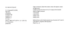
all Vr linspace 053100 figure1 ylim 0 2 xlim 025 3 xlabel Vr ylabel Pr Tr 09 Prfunc Vr 8Tr3 Vr 1 3Vr2 Pr ID: 572312
Download Presentation The PPT/PDF document "clc ; clear all; close" is the property of its rightful owner. Permission is granted to download and print the materials on this web site for personal, non-commercial use only, and to display it on your personal computer provided you do not modify the materials and that you retain all copyright notices contained in the materials. By downloading content from our website, you accept the terms of this agreement.
Slide1
clc; clear all; close allVr = linspace(0.5,3,100);figure(1);ylim([0 2])xlim([0.25 3])xlabel('V_r')ylabel('P_r')Tr = 0.9;Prfunc = @(Vr) 8*Tr./(3*Vr - 1) - 3./(Vr.^2);Pr = Prfunc(Vr);plot(Vr,Pr)
Clear command, clears the screen; clears all objects; closes all figures etc.
Creates values of
Vr
from 0.5 to 3 in steps of (3-0.5)/100
Opens a figure window
Y axis limits
X axis limits
Labels x axis
Labels y axis
Defines the van der Waals equation as a function of
Tr
and
Vr
Calculate
Pr
using the
vdW
equation
Plots
Pr
vs.
VrSlide2
if Tr < 1 Pr_b = 1.0; vdW_Pr_b = [1 -1/3*(1+8*Tr/Pr_b) 3/Pr_b -1/Pr_b]; Makes sure the temperature is below critical, Tr = T/TcStarts with a trial value for Pr at which liquid transform to gas
Defines a polynomial function to calculate the values of
Vr
for the trial value of Pr (Pr_b).The terms in the square brackets are the coefficients of the polynomial.
Slide3
v = sort(roots(vdW_Pr_b));A1 = (v(2)-v(1))*Pr_b - integral(Prfunc,v(1),v(2));A2 = integral(Prfunc,v(2),v(3)) - (v(3)-v(2))*Pr_b;Finds the roots of the polynomial and sorts them in increasing order: v(1), v(2), and v(3) Calculates the area enclosed by the line and the vdW curve between v(1) and v(2) and then from v(2) and v(3).(clearer figure later).Slide4
Z = abs(A1-A2);while Z > 0.0001 vdW_Pr_b = [1 -1/3*(1+8*Tr/Pr_b) 3/Pr_b -1/Pr_b]; v = sort(roots(vdW_Pr_b)); Prfunc = @(Vr) 8*Tr./(3*Vr - 1) - 3./(Vr.^2); A1 = (v(2)-v(1))*Pr_b - integral(Prfunc,v(1),v(2)); A2 = integral(Prfunc,v(2),v(3)) - (v(3)-v(2))*Pr_b; Z = abs(A1 - A2); Pr_b = Pr_b - 0.00001; figure(1); hold off; plot(Vr,Pr)
figure(1); hold on;
plot([0.5 3],[
Pr_b Pr_b],'k--') hold off; endCalculates the difference between the two areasIf z > 0.0001 then this loop startsDefines the polynomial in the loopCalculates and sorts the rootsDefines vdW equation in the loopCalculates the areas againCalculates the differenceLowers the test values Pr_b by 0.00001Chooses figure 1 window; new plot will appear, old graph is removedPlots Pr vs. VrChooses figure 1window; new plot will appear keeping the old graphPlots the line for Pr_b vs. Vr in a black dashed lineNext time a new graph is plotted the old plots will be removedStarts the loop again and checks if the difference between A1 and A2 (Z) > 0.0001 for the new value of Pr_b. Loop stops if Z < 0.0001 i.e A1 A2Slide5
Pr_bv(1)v(2)
v(3)
(v(2)-v(1))*Pr_b
(v(3)-v(2))*Pr_b Slide6
Pr_bv(1)v(2)
v(3)
integral(Prfunc,v(1),v(2))
integral(Prfunc,v(2),v(3))Calculates the area under the vdW curve from v(1) to v(2) and from v(2) to v(3).Slide7
Pr_bv(1)v(2)
v(3)
Calculates the relevant area for the Maxwell constructions
(v(2)-v(1))*Pr_b - integral(Prfunc,v(1),v(2))integral(Prfunc,v(2),v(3)) - (v(3)-v(2))*Pr_bSlide8
endA1A2Pr_bEnds the if loopPrints A1 and A2Prints the value of pressure Pr_b which satisfies Maxwell’s condition.