PDF-Example of Very Simple Path Analysis vi a Regression with correlation matrix input Entering PDF document

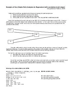
begin data mean 00 00 00 00 stddev 210 1500 325 125 n 300 300 300 300 corr 100 corr 30 100 corr 410 160 100 corr 330 570 500 100 end data brPage 2br Getting the

Upload by min-jolicoeur
Published on 2014-12-13

Presentation Embed Code

<iframe width="560" height="315" src="https://www.docslides.com/embed/23424" frameborder="0" allowfullscreen></iframe>

Download Presentation

Download Presentation The PPT/PDF document "Example of Very Simple Path Analysis vi ..." is the property of its rightful owner. Permission is granted to download and print the materials on this web site for personal, non-commercial use only, and to display it on your personal computer provided you do not modify the materials and that you retain all copyright notices contained in the materials. By downloading content from our website, you accept the terms of this agreement.