/
2/5/15 CMPS 3130/6130 Computational Geometry 2/5/15 CMPS 3130/6130 Computational Geometry

2/5/15 CMPS 3130/6130 Computational Geometry - PowerPoint Presentation

mindeeli
mindeeli . @mindeeli
Follow
343 views
Uploaded On 2020-06-23

2/5/15 CMPS 3130/6130 Computational Geometry - PPT Presentation

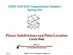
1 CMPS 31306130 Computational Geometry Spring 2015 Planar Subdivisions and Point Location Carola Wenk Based on Computational Geometry Algorithms and Applications and David Mounts lecture notes ID: 783737

cmps computational 6130 3130 computational cmps 3130 6130 geometry vertices time planar trapezoids segment vertex point face set trapezoid

Share:

Link:

Embed:

Download Presentation from below link

Download The PPT/PDF document "2/5/15 CMPS 3130/6130 Computational Geom..." is the property of its rightful owner. Permission is granted to download and print the materials on this web site for personal, non-commercial use only, and to display it on your personal computer provided you do not modify the materials and that you retain all copyright notices contained in the materials. By downloading content from our website, you accept the terms of this agreement.


Presentation Transcript

Slide1

2/5/15

CMPS 3130/6130 Computational Geometry

1

CMPS 3130/6130 Computational GeometrySpring 2015

Planar Subdivisions and Point LocationCarola WenkBased on:Computational Geometry: Algorithms and Applicationsand David Mount’s lecture notes

p

Slide2

2/5/15

CMPS 3130/6130 Computational Geometry

2

Planar SubdivisionLet

G=(V,E) be an undirected graph.G is planar if it can be embedded in the plane without edge crossings.

planar

K

5

, not planar

K

3,3

, not planar

A

planar embedding (=drawing) of a planar graph

G

induces a

planar subdivision

consisting of vertices, edges, and faces.

Slide3

2/5/15

CMPS 3130/6130 Computational Geometry

3

Doubly-Connected Edge List

The

doubly-connected edge list (DCEL) is a popular data structure to store the geometric and topological information of a planar subdivision.It contains records for each face, edge, vertex(Each record might also store additional application-dependent attribute information.)It should enable us to perform basic operations needed in algorithms, such as walk around a face, or walk from one face to a neighboring face

The DCEL consists of:

For each vertex

v

, its coordinates are stored in

Coordinates(

v

)

and a pointer

IncidentEdge

(

v

)

to a half-edge that has

v

as it origin.

Two oriented

half-edges per edge, one in each direction. These are called

twins. Each of them has an origin and a

destination. Each half-edge e

stores a pointer Origin(e), a pointer

Twin(e), a pointer

IncidentFace(e)

to the face that it bounds, and pointers Next (e)

and Prev(e)

to the next and previous half-edge on the boundary of IncidentFace(e

).

For each face f, OuterComponent

(f) is a pointer to some half-edge on its outer boundary (null for unbounded faces). It also stores a list

InnerComponents(f)

which contains for each hole in the face a pointer to some half-edge on the boundary of the hole.

Slide4

2/5/15

CMPS 3130/6130 Computational Geometry

4

Complexity of a Planar Subdivision

The complexity of a planar subdivision is: #vertices + #edges + #faces = nv + ne + nf

Euler’s formula for planar graphs:nv - n

e + nf

≥ 2n

e

≤ 3

n

v

– 6

2) follows from 1):

Count edges. Every face is bounded by

≥ 3

edges.

Every edge bounds

≤ 2

faces.

 3nf ≤ 2

ne  n

f ≤ 2/3ne

 2

≤ nv - n

e + nf

≤ nv - n

e + 2/3 ne

= nv – 1/3

ne

 2 ≤ nv – 1/3

ne

Hence, the complexity of a planar subdivision is O(n

v), i.e., linear in the number of vertices.

Slide5

2/5/15

CMPS 3130/6130 Computational Geometry

5

Point Location

Point location task: Preprocess a planar subdivision to efficiently answer point-location queries of the type: Given a point p=(

px,py), find the face it lies in.

p

Important metrics:

Time complexity for preprocessing

=

time to construct the data structure

Space

needed

to store the data structure

Time complexity for querying the data structure

Slide6

2/5/15

CMPS 3130/6130 Computational Geometry

6

Slab Method

Slab method: Draw a vertical line through each vertex. This decomposes the plane into slabs.

In each slab, the vertical order of the line segments remains constant.

If we know in which slab

p

lies, we can perform binary search, using the sorted order of the segments in the slab.

Find slab that contains

p

by binary search on

x

among slab boundaries.

A second binary search in slab determines the face containing

p

.

Search complexity

O(log

n

)

, but space complexity (n2

) .

p

p

p

lower bound?

Slide7

2/5/15

CMPS 3130/6130 Computational Geometry

7

Kirkpatrick’s Algorithm

Needs a triangulation as input.

Can convert a planar subdivision with

n

vertices into a triangulation:

Triangulate each face, keep same label as original face.

If the outer face is not a triangle:

Compute the convex hull of the subdivision.

Triangulate pockets between the subdivision and the convex hull.

Add a large triangle (new vertices

a

,

b

,

c

) around the convex hull, and triangulate the space in-between.

The size of the triangulated planar subdivision is still

O(

n

)

, by Euler’s formula.

The conversion can be done in

O(

n

log

n

)

time.

Given

p

, if we find a triangle containing

p we also know the (label of) the original subdivision face containing p.

a

b

c

p

Slide8

2/5/15

CMPS 3130/6130 Computational Geometry

8

Kirkpatrick’s Hierarchy

Compute a sequence

T

0, T1, …, T

k of increasingly coarser triangulations such that the last one has constant complexity.The sequence T

0

, T

1

, …, T

k

should have the following properties:

T

0

is the input triangulation,

Tk is the outer triangle

k  O(log

n)Each triangle in Ti+1 overlaps

O(1) triangles in Ti

How to build such a sequence?Need to delete vertices from Ti .

Vertex deletion creates holes, which needto be re-triangulated.How do we go from T

0 of size O(n) to

Tk of size O(1) in k=O(log

n) steps?In each step, delete a constant fractionof vertices from T

i .We also need to ensure that each new triangle in Ti+1 overlaps with only

O(1) triangles in Ti .

Slide9

2/5/15

CMPS 3130/6130 Computational Geometry

9

Vertex Deletion and Independent Sets

When creating

T

i+1

from

T

i

, delete vertices from

T

i

that have the following properties:

Constant degree:

Each vertex

v

to be deleted has

O(1)

degree in the graph

T

i

.

If

v

has degree

d

, the resulting hole can be re-triangulated with

d

-2 triangles

Each new triangle in

Ti+1 overlaps at most d

original triangles in Ti Independent sets:

No two deleted vertices are adjacent.Each hole can be re-triangulated independently.

Slide10

2/5/15

CMPS 3130/6130 Computational Geometry

10

Independent Set Lemma

Lemma:

Every planar graph on

n

vertices contains an independent vertex set of size

n

/18

in which each vertex has degree at most

8

. Such a set can be computed in

O(

n

)

time.

Use this lemma to construct Kirkpatrick’s hierarchy:

Start with

T

0

, and select an independent set

S

of size

n

/18

in which each vertex has maximum degree

8

. [Never pick the outer triangle vertices

a

,

b

, c.]Remove vertices of S, and re-triangulate holes.

The resulting triangulation, T1, has at most 17/18

n vertices.Repeat the process to build the hierarchy, until Tk equals the outer triangle with vertices a,

b, c.The depth of the hierarchy is k = log18/17 n

a

b

c

Slide11

2/5/15

CMPS 3130/6130 Computational Geometry

11

Hierarchy Example

Use this lemma to construct Kirkpatrick’s hierarchy:Start with T0, and select an independent set S of size

n/18 in which each vertex has maximum degree 8. [Never pick the outer triangle vertices a, b,

c.]Remove vertices of S, and re-triangulate holes.

The resulting triangulation, T1, has at most 17/18

n

vertices.

Repeat the process to build the hierarchy, until

T

k

equals the outer triangle with vertices

a

,

b

,

c

.The depth of the hierarchy is

k = log18

/17 n

Slide12

2/5/15

CMPS 3130/6130 Computational Geometry

12

Hierarchy Data Structure

Store the hierarchy as a DAG:The root is Tk . Nodes in each level correspond to triangles T

i .Each node for a triangle in Ti+1 stores pointers to all triangles of Ti that it overlaps.

How to locate point p in the DAG:

Start at the root. If p is outside of

T

k

then

p

is in exterior face; done.

Else, set

to be the triangle at the current level that contains

p

.

Check each of the at most 6 triangles of

T

k-1 that overlap with , whether they contain

p. Update  and descend in the hierarchy until reaching

T0 .Output

 .

p

Slide13

2/5/15

CMPS 3130/6130 Computational Geometry

13

Analysis

Query time is O(log n): There are O(log n) levels and it takes constant time to move between levels.Space complexity is O(n):Sum up sizes of all triangulations in hierarchy.

Because of Euler’s formula, it suffices to sum up the number of vertices.Total number of vertices:n + 17/18 n + (17/18)

2 n + (17/18)3 n + …

≤ 1/(1-17/18) n = 18

n

Preprocessing time

is

O(

n

log

n

)

:

Triangulating the subdivision takes

O(

n

log n

) time.The time to build the DAG is proportional to its size.

13

p

Slide14

2/5/15

CMPS 3130/6130 Computational Geometry

14

Independent Set Lemma

Lemma: Every planar graph on n vertices contains an independent vertex set of size n/18 in which each vertex has degree at most 8. Such a set can be computed in O(n) time.Proof:

Algorithm to construct independent set:Mark all vertices of degree ≥ 9

While there is an unmarked vertexLet v

be an unmarked vertexAdd

v

to the independent set

Mark

v

and all its neighbors

Can be implemented in

O(

n

)

time: Keep list of unmarked vertices, and store the triangulation in a data structure that allows finding neighbors in

O(1)

time.

v

Slide15

2/5/15

CMPS 3130/6130 Computational Geometry

15

Independent Set Lemma

Still need to prove existence of large independent set.Euler’s formula for a triangulated planar graph on n vertices: #edges = 3n – 6

Sum over vertex degrees: deg(

v) = 2 #edges = 6n

– 12 < 6n

Claim:

At least

n

/2

vertices have degree

≤ 8

.

Proof:

By contradiction. So, suppose otherwise.

n

/2

vertices have degree

≥ 9

. The remaining have degree

≥ 3.

 The sum of the degrees is ≥ 9 n/2 + 3

n/2 = 6n

. Contradiction.

In the beginning of the algorithm, at least n/2 nodes are unmarked. Each picked vertex

v marks ≤ 8 other vertices, so including itself

9. Therefore, the while loop can be repeated at least

n/18 times.

This shows that there is an independent set of size at least n/18 in which each node has degree

≤ 8.

v

Slide16

2/5/15

CMPS 3130/6130 Computational Geometry

16

Summing Up

Kirkpatrick’s point location data structure needs O(n log n) preprocessing time, O(n) space, and has O(log n)

query time.It involves high constant factors though.

Next we will discuss a randomized point location scheme (based on trapezoidal maps) which is more efficient in practice.

Slide17

2/5/15

CMPS 3130/6130 Computational Geometry

17

Trapezoidal map

Input: Set S={s1,…,sn}

of non-intersecting line segments.Query: Given point p, report the segment directly above

p.

Create trapezoidal map by shooting two rays vertically (up and down) from each vertex until a segment is hit. [Assume no segment is vertical.]

Trapezoidal map

= rays + segments

Enclose

S

into bounding box to avoid

infinite rays.

All faces in subdivision are trapezoids,

with vertical sides.

The trapezoidal map has at most

6

n

+4

vertices and

3

n

+1

trapezoids:Each vertex shoots two rays, so,

2n(1+2)

vertices, plus 4 for the bounding box.

Count trapezoids by vertex that creates itsleft boundary segment: Corner of box for

one trapezoid, right segment endpoint forone trapezoid, left segment endpoint for

at most two trapezoids.  3n

+1

Slide18

2/5/15

CMPS 3130/6130 Computational Geometry

18

Construction

Randomized incremental constructionStart with outer box which is a single trapezoid. Then add one segment si at a time, in random order.

s

i

Slide19

2/5/15

CMPS 3130/6130 Computational Geometry

19

Construction

Let Si={s1,…, si}, and let

Ti be the trapezoidal map for Si.

Add si

to Ti-

1

.

Find trapezoid containing left endpoint of

s

i

. [Point location;

details later

]

Thread

s

i

through

T

i-

1

, by walking through it and identifying trapezoids that are cut.“Fix trapezoids up” by shooting rays from left and right endpoint of

si and trim earlier rays that are cut by s

i.

s

i

Slide20

2/5/15

CMPS 3130/6130 Computational Geometry

20

Analysis

Observation:

The final trapezoidal map

T

i

does not depend on the order in which the segments were inserted.

Lemma:

Ignoring the time spent for point location, the insertion of

s

i

takes

O(

k

i

)

time, where

k

i

is the number of newly created trapezoids.

Proof:

Let

k

be the number of ray shots interrupted by

s

i

.

Each endpoint of

s

i

shoots two rays

k

i

=k+4 rays need to be processedIf k=0, we get 4 new trapezoids.Create a new trapezoid for each interrupted ray shot; takes O(1) time with DCELsisi

Slide21

2/5/15

CMPS 3130/6130 Computational Geometry

21

Analysis


1

2

3

n/2

n/2+1

n/2+2

n

Insert segments in

random

order:

P

= {all possible permutations/orders of segments};

|

P

| =

n

!

for

n

segments

k

i

=

k

i

(

p

)

for some random order

p

PWe will show that E(ki) = O(1)  Expected runtime E(T) = E(i=1ki) = i=1E(ki) = O(i=1 1) = O(n)

n

n

n

linearity of expectation

Slide22

2/5/15

CMPS 3130/6130 Computational Geometry

22

Analysis

Theorem: E(ki) = O(1), where k

i is the number of newly created trapezoids created upon insertion of si, and the expectation is taken over all segment

permutations of Si={

s1,…,

s

i

}

.

Proof:

T

i

does not depend on the order in which segments

s

1

,…,

s

i

were added.

Of s1,…,

si , what is the probability that a particular segment

s was added last?

1/i

We want to compute the number of trapezoids that would have been created if s was added last.

Slide23

2/5/15

CMPS 3130/6130 Computational Geometry

23

Analysis


Random variable ki(s)=

#trapezoids added when s was inserted

last in Si.

k

i

(s

)=

E(

k

i

)=


Slide24

2/5/15

CMPS 3130/6130 Computational Geometry

24

Analysis

Random variable

ki(s)=

#trapezoids added when s was inserted

last in Si

.

k

i

(s

)=

E(

k

i

)=

=

How many segments does

D

depend on? At most

4

.

Also,

T

i

has

O

(

i

)

trapezoids (by Euler’s formula).

E(

k

i

)=

=


Slide25

2/5/15

CMPS 3130/6130 Computational Geometry

25

Point Location

Build a point location data structure; a DAG, similar to Kirkpatrick’sDAG has two types of internal nodes:x-node (circle): contains the x-coordinate of a segment endpoint.

y-node (hexagon): pointer to a segmentThe DAG has one leaf for each trapezoid.

Children of

x

-node: Space to the left and right of

x

-coordinate

Children of

y

-node: Space above and below the segment

y

-node

is only searched when the query’s

x

-coordinate

is within the segment’s span.

Encodes trapezoidal decomposition and enables point location during construction.

Slide26

2/5/15

CMPS 3130/6130 Computational Geometry

26

Construction

Incremental construction during trapezoidal map construction.When a segment s is added, modify the DAG.

Some leaves will be replaced by new subtrees.Each old trapezoid will overlap

O(1) new trapezoids.

Each trapezoid appears exactly once as a leaf.

Changes are highly local.

If

s

passes entirely through trapezoid

t

, then

t

is replaced with two new trapezoids

t’

and

t’’

.

Add new

y

-node as parent of

t’ and t’’ , in order to facilitate search later.

If an endpoint of s

lies in trapezoid t, then add an x

-node to decide left/right and a y-node for the segment.

Slide27

2/5/15

CMPS 3130/6130 Computational Geometry

27

Inserting a Segment

Insert segment s3.

s3

s

3

p

3

q

3

p

3

q

3

Slide28

s3s

3

2/5/15

CMPS 3130/6130 Computational Geometry

28

Analysis

Space:

Expected

O

(

n

)

Size of data structure = number of trapezoids =

O

(

n

)

in expectation, since an expected

O

(1)

trapezoids are created during segment insertion

Query time:

Expected

O(log n

)Construction time:

Expected O(n log

n) follows from query time

Proof

that the query time is expected O(log

n):

Fix a query point Q.

Consider how Q moves through the trapezoidal map as it is being constructed as new segments are inserted.

Search complexity = number of trapezoids encountered by Q

Slide29

2/5/15

CMPS 3130/6130 Computational Geometry

29

Query Time

Let

Di be the trapezoid containing Q

after the insertion of ith segment.

If D

i

=

D

i-

1

then the insertion does not affect

Q

’s trapezoid (E.g.,

Q

B

).If D

i ≠

Di-1

then the insertion deleted Q

’s trapezoid, and Q needs to be located among the at most

4 new trapezoids.

Q

could fall 3 levels in the DAG.

s

3

s

3

Slide30

2/5/15

CMPS 3130/6130 Computational Geometry

30

Query Time

Let Xi be the # nodes on path created in iteration i, and

let Pi be the probability that there exists a node in iteration

i, i.e., Di

D

i-

1

The expected search path length

is

by lin. of expectation and since

Q

can drop at most

3

levels.

Claim:

P

i

≤ 4/

i

.

Backwards analysis: Consider deleting segments, instead of inserting.

Trapezoid

D

i

depends on

4

segments. The probability that the

ith segment is one of these 4 is

≤ 4/i .The expected search path length is at most Harmonic number  s3s3