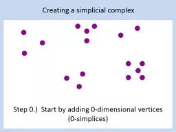
Step 0 Start by adding 0dimensional vertices 0simplices Creating a simplicial complex 1 A dding 1 dimensional edges 1simplices Add an edge between data points that are close ID: 558029
Download Presentation The PPT/PDF document "Creating a simplicial complex" is the property of its rightful owner. Permission is granted to download and print the materials on this web site for personal, non-commercial use only, and to display it on your personal computer provided you do not modify the materials and that you retain all copyright notices contained in the materials. By downloading content from our website, you accept the terms of this agreement.
Slide1
Creating a simplicial complex
Step 0.) Start by adding 0-dimensional vertices
(0-simplices)Slide2
Creating a simplicial complex
1
.)
A
dding
1
-dimensional edges (1-simplices)
Add an edge between data points that are “close”Slide3
Creating a simplicial complex
1
.)
A
dding
1
-dimensional edges (1-simplices)
Let T = Threshold
Connect vertices v and w with an edge
iff
the distance between v and w is less than TSlide4
Creating a simplicial complex
1
.)
A
dding
1
-dimensional edges (1-simplices)
Let T = Threshold =
Connect vertices v and w with an edge
iff
the distance between v and w is less than TSlide5
Creating a simplicial complex
1
.)
A
dding
1
-dimensional edges (1-simplices)
Add an edge between data points that are “close”
Note: we only need a definition of closeness between data points. The data points do not need to be actual points in
R
nSlide6
Creating the
Vietoris
Rips
simplicial complex
2
.) Add all possible simplices of dimensional > 1.Slide7
0.) Start by adding 0-dimensional data points
Use balls to measure distance
(Threshold = diameter).
Two points are close if their corresponding balls intersect
Creating the
Vietoris
Rips simplicial complexSlide8
0.) Start by adding 0-dimensional data points
Use balls of varying radii to determine persistence of clusters.
H.
Edelsbrunner
, D.
Letscher
, and A.
Zomorodian
, Topological persistence and
simplication
, Discrete and Computational Geometry 28, 2002, 511
-533.
Creating the
Vietoris
Rips simplicial complexSlide9
Constructing functional brain
networks with 97 regions of interest (ROIs) extracted from
FDG-PET data for 24 attention-deficit hyperactivity disorder (ADHD),
26 autism spectrum disorder (ASD) and11 pediatric control (PedCon).
Data = measurement fj taken at region j
Graph: 97 vertices representing 97 regions of interest edge exists between two vertices i,j if correlation between fj
and fj ≥ thresholdHow to choose the threshold?
Don’t, instead use persistent homology
Discriminative persistent homology of brain networks, 2011
Hyekyoung Lee
Chung, M.K.
;
Hyejin Kang
;
Bung-Nyun
Kim;Dong
Soo Lee Slide10Slide11
Vertices = Regions of Interest
Create Rips complex by growing epsilon balls (i.e. decreasing threshold) where distance between two vertices is given by
where fi
= measurement at location iSlide12
http://www.ima.umn.edu/videos/?id=856
http://ima.umn.edu/2008-2009/ND6.15-26.09/activities/Carlsson-Gunnar/imafive-handout4up.pdfSlide13
http://www.ima.umn.edu/videos/?id=1846
http://www.ima.umn.edu/2011-2012/W3.26-30.12/activities/Carlsson-Gunnar/imamachinefinal.pdf
Application to Natural Image Statistics
With V. de Silva, T. Ishkanov, A.
ZomorodianSlide14
An
image taken by black and white digital camera can
be viewed as a vector, with one coordinate for each pixelEach pixel has a “gray scale” value, can be thought of as a real number (in reality, takes one of 255 values
)Typical camera uses tens of thousands of pixels, so images lie in a very high dimensional space, call it pixel space, PSlide15
Lee
-Mumford-Pedersen [LMP] study only high
contrast patches.
Collection: 4.5 x 10⁶ high contrast patches from acollection of images obtained by van
Hateren and van der Schaaf
http://www.kyb.mpg.de/de/forschung/fg/bethgegroup/downloads/van-hateren-dataset.htmlSlide16
Lee
-Mumford-Pedersen [LMP] study only high
contrast patches.
Collection: 4.5 x 10⁶ high contrast patches from acollection of images obtained by van
Hateren and van der Schaaf
Choose how to model your dataSlide17
Choose how to model your data
Consult previous methods.Slide18
What to do if you are overwhelmed by the number of possible ways to model your data (or if you have no ideas):
Do what the experts do.Borrow ideas.
Use what others have done.Slide19
Carlsson
et al usedSlide20
Carlsson
et al used
The
majority of high-contrast
optical patches are concentrated around a 2-dimensional
C1 submanifold
embedded in the 7-dimensional
sphere.Slide21
0.) Start by adding 0-dimensional data points
Persistent Homology: Create the Rips complex
is a point in S
7
Slide22
For each fixed
e,
create Rips complex
from
the data
1
.)
A
dding
1
-dimensional edges (1-simplices)
Add an edge between data points that are close
is a point in
S
7
Slide23
For each fixed
e,
create Rips complex from the data
2
.) Add all possible simplices of dimensional > 1.
is a point in
S
7
Slide24
For each fixed
e,
create Rips complex from the
data
In reality used
Witness complex
(see later slides).
2
.) Add all possible simplices of dimensional > 1.
is a point in
S
7
Slide25
Probe the dataSlide26
Probe the dataSlide27
Can use function on data to probe the dataSlide28
Large values of
k:
measuring density
of large neighborhoods of
x, S
maller values mean we are using smaller neighborhoodsSlide29
Eurographics
Symposium on Point-Based Graphics (2004)
Topological estimation using witness complexesVin de Silva and Gunnar CarlssonSlide30
Eurographics
Symposium on Point-Based Graphics (2004)
Topological estimation using witness complexesVin de Silva and Gunnar CarlssonSlide31Slide32Slide33Slide34Slide35Slide36
From:
http
://plus.maths.org/content/imaging-maths-inside-
klein-bottleFrom: http://
www.math.osu.edu/~fiedorowicz.1/math655/Klein2.htmlKlein BottleSlide37
M(100, 10) U Q
where |Q| = 30
On
the Local Behavior of Spaces of Natural Images, Gunnar Carlsson, Tigran Ishkhanov, Vin de Silva,
Afra Zomorodian, International Journal of Computer Vision 2008, pp 1-12.Slide38
http://www.maths.ed.ac.uk/~
aar/papers/ghristeat.pdfSlide39
http://
www.nsf.gov/discoveries/disc_summ.jsp?cntn_id=112392Slide40
Combine your analysis with other toolsSlide41