George Williams described Mother Nature as a “Wicked Old Witch” - PowerPoint Presentation

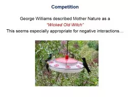
George Williams described Mother Nature as a “Wicked Old Witch” This seems especially appropriate for negative interactions… Competition

Competition Competition (generally an intra-trophic level phenomenon) occurs when each species negatively influences the population growth rate (or size) of the other This phenomenological definition is used in the modeling framework proposed by Alfred Lotka (1880-1949) & Vito Volterra (1860-1940) Their shared goal was to determine the conditions under which competitive exclusion vs. coexistence would occur between two sympatric competitors

N Time Exponential growth ∆N ∆t = r • N Occurs when growth rate is proportional to population size; Requires unlimited resources Population Dynamics

N Density-dependent per capita birth (b) b d r Equilibrium (= carrying capacity, K) & death (d) rates or d b Notice that per capita fitness increases with decreases in population size from K Population Dynamics

N Time Logistic growth ∆N ∆t = r • N • (1 – ) N K K = carrying capacity ∆N ∆t is maximized ∆N ∆t = 0 ∆N ∆t = 0 Population Dynamics

In the logistic population growth model , the growth rate is reduced by intraspecific competition: Species 1: dN1/dt = r1N1[(K1-N1)/K1] Species 2: dN2/dt = r 2N2[(K2-N2)/K2]Lotka & Volterra’s equations include functions to further reduce growth rates as a consequence of interspecific competition : Species 1: dN 1 /dt = r 1 N1[(K1-N1-f (N2))/K1] Species 2: dN2/dt = r2N2[(K2-N2-f(N 1))/K2] Lotka-Volterra Competition Equations: Competition

Lotka-Volterra Competition Equations: The function ( f ) could take on many forms, e.g.: Species 1: dN1/dt = r1N1[(K1-N1-αN2)/K1] Species 2: dN2/dt = r2N2[(K2 -N 2 - β N 1 )/K2] The competition coefficients α & β measure the per capita effect of one species on the population growth of the other, measured relative to the effect of intraspecific competition If α = 1, then per capita intraspecific effects = interspecific effects If α < 1, then intraspecific effects are more deleterious to Species 1 than interspecific effects If α > 1, then interspecific effects are more deleterious Competition

2 2 2 2 1 1 1 1 Area within the frame represents carrying capacity (K) of either species 1 1 1 1 1 The size of each square is proportional to the resources an individual consumes and makes unavailable to others (Sp. 1 = purple, Sp. 2 = green) Individuals of Sp. 2 consume 4x resources consumed by individuals of Sp. 1 For Species 1: dN 1 /dt = r 1 N 1 [(K 1 -N 1 - α N 2 )/K 1 ] … where α = 4. Redrawn from Gotelli (2001)

2 2 2 2 1 1 1 1 Competition is occurring because both α & β > 0  α = 4 & β = ¼ 1 1 1 1 1 In this case, adding an individual of Species 2 is more deleterious to Species 1 than is adding an individual of Species 1… but, adding an individual of Species 1 is less deleterious to Species 2 than is adding an individual of Species 2 Redrawn from Gotelli (2001)

2 2 2 2 1 1 1 1 1 1 1 1 1 Asymmetric competition In this case: α > β α > 1 β < 1

Asymmetric competition can occur throughout the spectrum of: α  β, (α < = > 1, or β < = > 1) 2 2 2 2 1 1 1 What circumstances might the figure above represent? Exclusively interspecific territoriality, intra-guild predation… Asymmetric competition In this case: α > β α > 1 β = 1

In this case: α = β = 1, i.e., the special case of competitive equivalence Symmetric competition can occur throughout the spectrum of:(α = β) < = > 1 2 2 2 2 1 1 1 Symmetric competition

This makes intuitive sense: The equilibrium for N 1 is the carrying capacity for Species 1 (K 1 ) reduced by some amount owing to the presence of Species 2 (α N2) Find equilibrium solutions to the equations, i.e., set dN/dt = 0: Species 1: N1 = K1 - αN2 Species 2: N2 = K2 - βN1 ^ ^ ^ ^ However, each species’ equilibrium depends on the equilibrium of the other species! So, by substitution… Species 1: N 1 = K 1 - α (K 2 - β N 1 ) Species 2: N 2 = K 2 - β (K 1 - αN2) ^ ^Lotka-Volterra Phenomenological Competition Model

These provide some insights into the conditions required for coexistence under the assumptions of the model The equations for equilibrium solutions become: Species 1: N 1 = [K 1 - αK2] / [1 - α β] Species 2: N2 = [K2 - βK1] / [1 - α β] ^ ^ E.g ., the product αβ must be < 1 for N to be > 0 for both species (a necessary condition for coexistence) But they do not provide much insight into the dynamics of competitive interactions, e.g. , are the equilibrium points stable? Lotka-Volterra Phenomenological Competition Model

State-space graphs help to track population trajectories (and assess stability) predicted by models Mapping state-space trajectories onto single population trajectories 4 time steps From Gotelli (2001)

State-space graphs help to track population trajectories (and assess stability) predicted by models Mapping state-space trajectories onto single population trajectories 4 time steps 4 time steps From Gotelli (2001)

Remember that equilibrium solutions require dN/dt = 0 Species 1: N 1 = K 1 - αN2 Isocline for Species 1dN1/dt = 0 ^ N 1 N 2 K 1 K 1 / α Therefore: When N 2 = 0, N 1 = K 1 When N 1 = 0, N 2 = K 1 / α Lotka-Volterra Model

Remember that equilibrium solutions require dN/dt = 0 Species 2: N 2 = K 2 - βN1 ^ N 1 N 2 K 2 / β K 2 Isocline for Species 2 dN 2 /dt = 0 Therefore: When N 1 = 0, N 2 = K 2 When N 2 = 0, N 1 = K 2 / β Lotka-Volterra Model

N 2 K 2 / β K 2 Plot the isoclines for 2 species together to examine population trajectories K 1 / α > K 2 K1 > K2/ β For species 1: K1 > K2α (intrasp. > intersp.)For species 2: K1β > K2 (intersp. > intrasp.) K 1 K 1 / α = stable equilibrium Competitive exclusion of Species 2 by Species 1 Lotka-Volterra Model N 1

N 2 K 2 / β K 1 / α Plot the isoclines for 2 species together to examine population trajectories K 2 > K 1 /αK 2/β > K 1For species 1: K2α > K1 (intersp. > intrasp.)For species 2: K2 > K1 β (intrasp. > intersp.) K 1 K 2 Competitive exclusion of Species 1 by Species 2 = stable equilibrium Lotka-Volterra Model N 1

N 2 K 2 / β K 1 / α Plot the isoclines for 2 species together to examine population trajectories K 2 > K 1 / α K1 > K2/β For species 1: K 2 α > K 1 (intersp. > intrasp.) For species 2: K 1 β > K2 (intersp. > intrasp.) K 1 K 2 Competitive exclusion in an unstable equilibrium = stable equilibrium = unstable equilibrium Lotka-Volterra Model N 1

N 2 K 2 / β K 2 Plot the isoclines for 2 species together to examine population trajectories K 1 / α > K 2 K2/β > K1 For species 1: K 1 > K2α (intrasp. > intersp.)For species 2: K2 > K1β (intrasp. > intersp.) K 1 K 1 / α = stable equilibrium Coexistence in a stable equilibrium Lotka-Volterra Model N 1

Earliest experiments within the Lotka-Volterra framework: Gause (1932) – protozoans exploiting cultures of bacteria The Lotka-Volterra models, coupled with the results of simple experiments suggested a general principle in ecology: The Lotka-Volterra-Gause Competitive Exclusion Principle “Complete competitors cannot coexist” (Hardin 1960) Competition Major prediction of the Lotka-Volterra competition model: Two species can only stably coexist if intraspecific competition is stronger than interspecific competition for both species

Competition The Lotka-Volterra equations have been used extensively to model and better understand competition, but they are phenomenological and completely ignore the mechanisms of competitionIn other words, they ignore the question: Why does a particular interaction between species mutually reduce their population growth rates and depress population sizes?

Competition A commonly used, binary classification of mechanisms: Exploitative / scramble (mutual depletion of shared resources) Interference / contest (direct interactions between competitors)More detailed classification of mechanisms (from Schoener 1983): Consumptive (comp. for resources) Preemptive (comp. for space; a.k.a. founder control ) Overgrowth (cf. size-asymmetric competition of Weiner 1990) Chemical (e.g., allelopathy) Territorial Encounter Exploitative / consumptive further divided by Byers (2000): Resource suppression due to consumption rate Resource-conversion efficiency

Competition Case & Gilpin (1975) and Roughgarden (1983) claimed that interference competition should not evolve unless exploitative competition exists between two species Why?Interference competition is costly, and is unlikely to evolve under conditions in which there is no payoff. If the two species do not potentially compete for limiting resources (i.e., there is no opportunity for exploitative competition), then there would be no reward for engaging in interference competition.

Resource, R dN/ N * dt ( per capita ) Species A m A R * Per capita reproductive rate of Species 1 ( dN/(N *dt) ) is a function of resource availability, R Mortality rate, m A , is assumed to remain constant with changing R R* = equilibrium resource availability at which reproduction and mortality are balanced, and the level to which species A can reduce R in the environment Tilman’s Resource-Based Competition Models

Resource, R Species A Species B m B m A R B R A * * When two species compete for one limiting resource , the species with the lower R* deterministically outcompetes the other Species B wins in this case dN/ N * dt ( per capita ) Tilman’s Resource-Based Competition Models

R 1 R 1 * dN/dt > 0 dN/dt < 0 Now consider the growth response of one species to two essential resources R* divides the region into portions favorable and unfavorable to population growth Tilman’s Resource-Based Competition Models

R 1 R 2 * R 1 * R 2 dN/dt > 0 dN/dt < 0 Now consider the growth response of one species to two essential resources R* divides the region into portions favorable and unfavorable to population growth Tilman’s Resource-Based Competition Models

R 1 R 2 * R 1 * R 2 dN/dt > 0 dN/dt < 0 Zero Net Growth Isocline (ZNGI) Resource supply point Consumption vector Now consider the growth response of one species to two essential resources The two R*s divide the region into portions favorable and unfavorable to population growth Consumption vectors can be of any slope, but the slope predicted under optimal foraging would equal R 2 /R 1 * * If a population deviates from the equilibrium along the ZNGI, it will return to the equilibrium Tilman’s Resource-Based Competition Models

R 1 Now consider two species potentially competing for two essential resources R 2 A B 1 2 3 In this case, species A outcompetes species B in habitats 2 & 3, and neither species can persist in habitat 1 Tilman’s Resource-Based Competition Models

R 1 R 2 A B 1 2 ? 6 Resource supply points In this case, species A wins in habitat 2, species B wins in habitat 6, and neither species can persist in habitat 1 Consumption vectors Tilman’s Resource-Based Competition Models

R 1 There is also an equilibrium point at which both species can coexist The extent to which that equilibrium is stable depends on the relative consumption rates of the two species consuming the two resources R 2 A B 1 2 ? 6 Tilman’s Resource-Based Competition Models

R 1 R 2 A B 1 2 3 4 5 6 Slope of consumption vectors for A Slope of consumption vectors for B The extent to which that equilibrium is stable depends on the relative consumption rates of the two species consuming the two resources In this case, it is stable Tilman’s Resource-Based Competition Models

R 1 The extent to which that equilibrium is stable depends on the relative consumption rates of the two species consuming the two resources In this case, it is stable Species A can only reduce R2 to a level that limits species A, but not species B, whereas species B can only reduce R1 to a level that limits species B, but not species A R 2 A B 1 2 3 4 5 6 Resource supply point Consumption vectors Slope of consumption vectors for A Slope of consumption vectors for B Each species will return to its equilibrium if displaced on its ZNGI Tilman’s Resource-Based Competition Models

R 1 R 2 A B 1 2 3 4 5 6 The extent to which that equilibrium is stable depends on the relative consumption rates of the two species consuming the two resources In this case, it is unstable Slope of consumption vectors for B Slope of consumption vectors for A Tilman’s Resource-Based Competition Models

R 1 R 2 A B 1 2 3 4 5 6 The extent to which that equilibrium is stable depends on the relative consumption rates of the two species consuming the two resources In this case, it is unstable Species A can reduce R 1 to a level that limits species A and excludes species B, whereas species B can reduce R 2 to a level that limits species B and excludes species A Slope of consumption vectors for B Slope of consumption vectors for A Resource supply point Consumption vectors Each species will return to its equilibrium if displaced on its ZNGI Tilman’s Resource-Based Competition Models

Competition The Lotka-Volterra competition model and Tilman’s R* model are both examples of mean-field, analytical models (a.k.a. “general strategic models”) Neighborhood models describe how individual organisms respond to variation in abundance or identity of neighbors “ In sessile organisms such as plants, competition for resources occurs primarily between closely neighboring individuals ” Antonovics & Levin (1980) How relevant is the mean-field assumption to real organisms?

Competition Spatially Explicit, Neighborhood Models of Plant Competition There are many ways to formulate these models, and most require computer-intensive simulations: Cellular automata – Start with a grid of cells… Spatially explicit individual-based models – Keep track of the demographic fate and spatial location of every individual in the population Sometimes these are “ empirical, field-calibrated models”

Competition A key conclusion of these models: At highest dispersal rates, i.e ., “ bath dispersal”, the predictions of the mean-field approximations are often matched by the predictions of the more complicated, spatially-explicit modelsSpatially Explicit, Neighborhood Models of Plant Competition Low dispersal rates, however, lead to intraspecific clumping , which tends to relax (broaden) the conditions under which two-species coexistence occurs; this is similar to increasing the likelihood of intraspecific competition relative to interspecific competition

Competition Connell (1983) Reviewed 54 studies 45/54 (83%) were consistent with competition Of 54 studies, 33 (61%) suggested asymmetric competition Schoener (1983) Reviewed 164 studies 148/164 (90%) were consistent with competition Of 61 studies, 51 (85%) suggested asymmetric competition Kelly, Tripler & Pacala (ms. 1993) [But apparently never published!] Only 1/4 of plot-based studies were consistent with competition, whereas 2/3 of plant-centered studies were consistent with competition

A classic competition study: MacArthur (1958) Five sympatric warbler species with similar bill sizes and shapes broadly overlap in arthropod diet, but they forage in different zones within spruce crowns Is this an example of the “ ghost of competition past ” ( sensu Connell [1980])?

Competition between seed-eating rodents and ants in the Chihuahuan Desert Brown & Davidson (1977) Strong resource limitation – seeds are the primary food of many taxa (rodents, birds, ants) Almost complete overlap in the sizes of seeds consumed by ants and rodents – demonstrates the potential for strong competition Design: Long-term exclosure experiments – fences to exclude rodents, and insecticide to remove ants; re-censuses of ant and rodent populations through time Results and Conclusion: Excluded rodents and the number of ant colonies increased 70% Excluded ants and rodent biomass increased 24% Competition can apparently occur between distantly related taxa

Competition between sexual and asexual species of geckoPetren et al. (1993) Humans have aided the dispersal of a sexual species of gecko ( Hemidactylus frenatus ) to several south Pacific islands and it is apparently displacing asexual species Lepidodactylus lugubris,asexual native on south Pacific islands Results and Conclusion: L. lugubris avoids H. frenatus at high concentrations of insects on lighted walls Sometimes “obvious” hypothesized reasons for competitive dominance are incorrect Experiment: Added H. frenatus and L. lugubris alone and together to aircraft hanger walls

Competition among Anolis lizards (Pacala & Roughgarden 1982) What is the relationship between the strength of interspecific competition and degree of interspecific resource partitioning? 2 pairs of abundant insectivorous diurnal Anolis lizards on 2 Caribbean islands: St. Maarten: A. gingivinus & A. wattsi pogusSt. Eustatius: A. bimaculatus & A. wattsi schwartzi

Competition among Anolis lizards (Pacala & Roughgarden 1982) Body size (strongly correlated with prey size): St. Maarten anoles: large overlap in body size St. Eustatius anoles: small overlap in body sizeForaging location: St. Maarten anoles: large overlap in perch ht. St. Eustatius anoles: no overlap in perch ht. Experiment:Replicated enclosures on both islands, stocked with one (not A. wattsi) or both species

Results and Conclusions: St. Maarten (similar resource use) Growth rate of A. gingivinus was halved in the presence of A. wattsiSt. Eustatius (dissimilar resource use) No effect of A. wattsi on growth or perch height of A. bimaculatisStrength of present-day competition in these species pairs is inversely related to resource partitioning Competition among Anolis lizards (Pacala & Roughgarden 1982)

Why do these pairs of anoles on nearby islands (30 km) differ in degree of resource partitioning? Hypothesis: Character displacement occurred on St. Eustatius during long co-evolutionary history ( i.e ., the ghost of competition past), whereas colonization of St. Maarten occurred much more recently, and in both cases colonization was by similarly sized Anolis speciesCharacter displacement:Evolutionary divergence of traits in response to competition, resulting in a reduction in the intensity of competition Competition among Anolis lizards (Pacala & Roughgarden 1982)

Pacala & Roughgarden (1985) presented evidence to suggest that both species pairs have a long history of co-occurrence on their respective islands and that different colonization histories resulted in the observed patterns of resource partitioning Both islands may have been colonized by Anolis species differing in size, yet on St. Maarten the larger Anolis colonized later and has subsequently converged in body size on the smaller residentCompetition among Anolis lizards (Pacala & Roughgarden 1985)

Character Displacement Schluter & McPhail (1992) surveyed the literature on character displacement and listed criteria necessary to exclude other potential explanations for species that share similar traits in allopatry, but differ in sympatry (similar to Connell’s [1980] requirements to demonstrate the “ghost of competition past”):1. Chance should be ruled out as an explanation for the pattern (appropriate statistical tests, often involving null models) 2. Phenotypic differences should have a genetic basis 3. Enhanced differences between sympatric species should be the outcome of evolutionary shifts, not simply the inability of similar-sized species to coexist 4. Morphological differences should reflect differences in resource use 6. Independent evidence should be obtained that similar phenotypes actually compete for food 5. Sites of sympatry and allopatry should be similar in terms of physical characteristics