Robin Lock Burry Professor of Statistics St Lawrence University AMATYC Webinar December 6 2016 The Lock 5 Team Patti amp Robin St Lawrence Kari Harvard Penn State Eric North Carolina ID: 759377
Download Presentation The PPT/PDF document "Bootstraps An Intuitive Introduction to ..." is the property of its rightful owner. Permission is granted to download and print the materials on this web site for personal, non-commercial use only, and to display it on your personal computer provided you do not modify the materials and that you retain all copyright notices contained in the materials. By downloading content from our website, you accept the terms of this agreement.
Slide1
BootstrapsAn Intuitive Introduction to Confidence Intervals
Robin Lock
Burry Professor of Statistics
St. Lawrence University
AMATYC Webinar
December 6, 2016
Slide2The Lock
5 Team
Patti & RobinSt. Lawrence
KariHarvardPenn State
EricNorth CarolinaMinnesota
Dennis
Iowa State
Miami Dolphins
Slide3Two Approaches to Inference
Traditional: Assume some distribution (e.g. normal or t) to describe the behavior of sample statisticsEstimate parameters for that distribution from sample statisticsCalculate the desired quantities from the theoretical distribution
Simulation (SBI):
Generate many samples (by computer) to show the behavior of sample statistics
Calculate the desired quantities from the simulation distribution
Slide4Simulation-Based Inference (SBI) Projects
Lock5 lock5stat.com Tintle, et al math.hope.edu/isi Catalst www.tc.umn.edu/~catalstTabor/Franklin www.highschool.bfwpub.comOpen Intro www.openintro.org
Slide5Intro Stat – Revised Topics
Descriptive Statistics – one and two samples
Normal distributions
Data production (samples/experiments)
Sampling distributions (mean/proportion)
Confidence intervals (means/proportions)
Hypothesis tests (means/proportions)
ANOVA for several means, Inference for regression, Chi-square tests
Data production (samples/experiments)
Bootstrap confidence intervals
Randomization-based hypothesis tests
Normal distributions
Bootstrap confidence intervals
Randomization-based hypothesis tests
Descriptive Statistics – one and two samples
Slide6Intro Stat – Revised Topics
Confidence intervals (means/proportions)
Hypothesis tests (means/proportions)
ANOVA for several means, Inference for regression, Chi-square tests
Data production (samples/experiments)
Normal distributions
Bootstrap confidence intervals
Randomization-based hypothesis tests
Descriptive Statistics – one and two samples
See the April 7, 2016 AMATYC Webinar on “Teaching Introductory Statistics with Simulation-Base Inference”
by Allan Rossman and Beth Chance
Slide7Intro Stat – Revised Topics
Confidence intervals (means/proportions)
Hypothesis tests (means/proportions)
ANOVA for several means, Inference for regression, Chi-square tests
Data production (samples/experiments)
Normal distributions
Bootstrap confidence intervals
Randomization-based hypothesis tests
Descriptive Statistics – one and two samples
See the rest of THIS webinar!
Slide8Questions to Address
What is bootstrapping?
How can we use bootstrapping to find confidence intervals?
Can bootstrapping be made accessible to intro statistics students?
Can it be used as a way to
introduce
students to key ideas of confidence intervals?
Why does bootstrapping work?
What about traditional methods?
Slide9Where are we in the course?
Data Production: Random sampling, random assignment
Students have seen…
Graphical Displays:
Summary Statistics:
How accurate are these estimates?
Slide10Example #1: What is the average price of a used Mustang car?
A student selects a random sample of n=25 Mustangs from a website (autotrader.com) and records the price (in $1,000’s) for each car.
Slide11Sample of Mustangs:
Our best estimate for the average price of used Mustangs is $15,980, but how accurate is that estimate?
Key idea:
How much do we expect the mean price to vary when we take samples of 25 cars at a time?
Goal:
Find an interval that is likely to contain the mean price for
all
Mustangs
Confidence Interval
Slide12Traditional Inference
2. Which formula?
3. Calculate summary stats
6. Plug and chug
4. Find t
*
5.
df
?
df=251=24
t
*=2.064
7. Interpret in context
CI for a mean
1. Check conditions
“We are 95% confident that the mean price of all used Mustang cars at this site is between $11,390 and $20,570.”
n
= 25
Slide13Answer is fine, but the process is not very helpful at building understanding of a CI. Can we arrive at the same answer in a way that also builds understanding?
Traditional Inference
(yes!)
Slide14Key Concept: How much do sample statistics vary?
If we take samples of 25 Mustangs at a time, what sort of distribution should we expect to see for ?
Sampling Distribution of
Producing a Sampling Distribution
Possible traditional approaches:Know the value of the parameter and distribution of the populationTake thousands of samples from the populationRely on theoretical approximations
and (2) are not practical in real situations
(3) is difficult for introductory students
Slide16Key Concept: How much do sample statistics vary?
Bootstrap!!!
How can we figure out how much sample statistics vary when we only have ONE sample?
Slide17Bootstrapping
Brad
Efron Stanford University
Key idea:
Take many samples with replacement from the original sample using the same n to see how the statistic varies.
Assumes the “population” is many, many copies of the original sample.
Slide18Original Sample (
n=6)
Finding a Bootstrap Sample
A simulated “population” to sample from
Bootstrap Sample: (sample
with replacement
from the original sample)
Slide19Original Sample
Bootstrap Sample
Repeat 1,000’s of times!
Slide20Many times
Original Sample
BootstrapSample
BootstrapSample
BootstrapSample
●
●
●
Bootstrap Statistic
Sample Statistic
Bootstrap Statistic
Bootstrap Statistic
●
●
●
Bootstrap Distribution
We need technology
!
Slide21lock5stat.com/statkey
StatKey
Freely available web apps with no login required
Runs in (almost) any browser (incl. smartphones/tablets)
Google Chrome App available (no internet needed)
Use standalone or supplement to existing technology
Slide22lock5stat.com/
statkey
Slide23Bootstrap Distribution for Mustang Price Means
Slide24How do we get a CI from the bootstrap distribution?
Method #1: Standard ErrorFind the standard error (SE) as the standard deviation of the bootstrap statisticsFind an interval with
Standard Error
)
How do we get a CI from the bootstrap distribution?
Method #1: Standard ErrorFind the standard error (SE) as the standard deviation of the bootstrap statisticsFind an interval with
Method #2: Percentile Interval
For a 95% interval, find the endpoints that cut off 2.5% of the bootstrap means from each tail, leaving 95% in the middle
Slide2795% CI via Percentiles
Keep 95% in middle
Chop 2.5% in each tail
We are 95% sure that the mean price for Mustangs is between $11,918 and $20,290
Slide2899% CI via Percentiles
Keep 99% in middle
Chop 0.5% in each tail
We are 99% sure that the mean price for Mustangs is between $10,878 and $21,502
Slide29Bootstrap Confidence IntervalsVersion 1 (Statistic 2 SE): Great preparation for moving to traditional methodsVersion 2 (Percentiles): Great at building understanding of confidence level
Same
process works for different parameters
Slide30Brief pause for questions so far?
Slide31Example #2: What proportion of statistics students use a Mac?
A sample of n=172 stat students contains 118 that use a Mac.
How accurate is that sample proportion?
Find a 95% confidence interval for the proportion of all statistics students that use a Mac.
Slide32Bootstrap distribution for
We are 95% sure that the proportion of stat students with Macs is between 0.616 and 0.756.
Example #3: Find a 95% CI for the difference in average Math SAT score between female and male stat students.
Example #4: Find a 90% CI for the standard deviation of Math SAT score for stat students.
Data: StudentSurvey.csv available at http://lock5stat.com
Slide34Transition to Traditional Methods
for Mustang prices
for Mac owners
for Math SAT
for Math SAT
All symmetric bell-shapes!
Slide35Normal Distribution
Slide36This is where the “2” comes from
where z* comes from the normal distribution to give the desired confidence.
N(0,1)
Slide37Formulas for SE
We complete the transition to a traditional (formula) CI, IF (a) We have a formula to compute the SE (b) We have conditions to know the distribution
Example: CI for p
Normal if
and
Verifying with Bootstraps
Why
does the bootstrap work?
Sampling Distribution
Population
µ
BUT, in practice we don’t see the “tree” or all of the “seeds” – we only have ONE seed
Slide41Bootstrap Distribution
Bootstrap
“Population”
What can we do with just one seed?
Grow a NEW tree!
Estimate the distribution and variability (SE) of
’s from the bootstraps
µ
Use the bootstrap errors that we CAN see to estimate the sampling errors that we CAN’T see.
Slide42Golden Rule of Bootstraps
The
bootstrap statistics
are to the
original statistic
as
the
original statistic
is to the
population parameter
.
Slide43Final Thoughts
The bootstrap approach is a way to introduce students to the main ideas of confidence intervals, while requiring only minimal background knowledge of sampling and summary statistics.The methods are easily generalized to lots of parameter situations. Use of the bootstrap distribution appeals to visual learners. Some technology (e.g. StatKey) is needed.Techniques lead smoothly into traditional methods.
Thanks for Listening!
rlock@stlawu.edu
lock5stat.com
Thanks for listening!
rlock@stlawu.edu
lock5stat.com