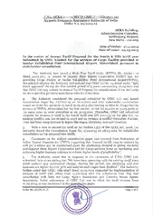
Generation Computing, 13 (1995) 245-286 OHMSHA, LTD. and Springer-Verl - PDF document

Generation Computing, 13 (1995) 245-286 OHMSHA, LTD. and Springer-Verlag A,  OHMSHA, LTD. 1995 Entailment and Progol MUGGLETON Oxford University Computing Laboratory, Wolfson Building, Parks Road, Received 3 October 1994 Revised manuscript received 2 April 1995 Abstract This paper firstly provides a re-appraisal of the develop- ment of techniques for inverting deduction, secondly introduces Mode- Keywords: Learning, Logic Programming, Induction, Predicate Invention, Inverse Resolution, Inverse Entailment, Information Introduction its inception in this journal 31) Inductive Logic Programming (ILP) has grown to become a substantial sub-area of both Machine Learning and Logic Programming (see Ref. 43)). The success of S. Muggleton include the problem of inverting resolution, a7'61'~4) inversion of clausal implication, zz'~4'~~ predicate invention, 36) closed-world specialisation 1) and U-learnability. 4z) As with any subject, the diversity of sub-topics can be better understood by following the development of a particular line of ideas. The aims of this paper are firstly to provide a re-appraisal of the development of tech- niques for inverting deduction, secondly to introduce Mode-Directed Inverse Entailment (MDIE) as a generalisation and enhancement of previous approaches and thirdly to describe an implementation of MDIE in the Progol* system. At each stage in the development of ILP there has been an attempt to solve existing technical restrictions of implemented systems. The five main approaches described in this paper are as follows. (1) Inverse resolution (IR) in propositional logic, (2) IR in first-order definite clause logic, (3) determinate relative least general generalisation, (4) inverse implication and (5) mode-directed inverse entailment. The paper is structured as follows. First the logical and statistical setting for ILP are introduced (Section 2). This is followed by a synopsis of the results and restrictions for approaches (1) to (4) (Sections 3 to 6). The remainder of the paper (Sections 7 to 12) deals with theoretical and practical aspects of mode- directed inverse entailment. Instructions for obtaining Progol by anonymous ftp are given in Section ll. The paper closes with a discussion of research issues related to inverse entailment. Standard definitions taken from Logic Program- ming and ILP are given in Appendix A. In Appendix B a statistical setting for ILP is described. Properties of the subsumption lattice are described in Appen- dix C. The algorithms used in Progol are given in Appendix D. A table of Progol's runtimes various data sets is presented in Appendix E. Logical and Statistical Setting for ILP inference derives consequences E from a prior theory T. Thus if T says that all swans are white, E might state that a particular swan is white. Inductive inference derives a general belief T from specific beliefs E. After observing one or more white swans T might be the conjecture that all swans are white. In both deduction and induction T and E must be consistent and T ~ E. (1) The requirement of consistency means that the observation of a black swan rules out conjecture T. Inductive inference is, in a sense, the inverse of deduction. However, deductive inference proceeds by application of sound rules of infer- Prolog inverted in the middle. Entailment and Progol while inductive inference necessarily involves unsound conjecture. Such conjectures have at best statistical support from observed data. However, the association of probability values with hypotheses requires the assumption of a prior probability distribution over the hypothesis language. Occam's razor can be taken as an instance of a distribution which assigns higher prior probability to simpler hypotheses. It has been shown 4) that without such distributional assumptions the class of all logic programs is not even PAC-predictable. On the other hand, it has recently been demonstrated 42) that the class of all time- bounded logic programs is polynomial-time learnable (U-learnable) under fairly broad families of prior probability distributions. Appendix B gives more details of the relationship between data, posterior probabilities and U-learnability. Within ILP it is usual to separate the elements of (1) into examples (E), background knowledge (B), and hypothesis (H). These have the relationship A H ~ E. (2) H and E are each logic programs. E usually contains ground unit clauses of a single target predicate. E can be separated into E +, ground unit definite clauses and E-, ground unit headless Horn clauses. However, the separation into B, H and E is a matter of convenience, as the following example shows. 1 White swans swan example might be represented using the following logic program. E+ = { white(swanl) +- swan(swanl) +- black(swan2) ~-- E- = swan(swan2) ~-- B -- { ~---black(X), white(X) H = { white(X) ~ swan(X) Relationship (2) does not hold since swan(swanl) is not entailed by B /~ H. It does not help to argue that swan(swanl) is background knowledge, since this is an observations about swanl. E- does not contain headless Horn clauses, although together with B it refutes H. These problems can most simply be avoided by dropping all but the restriction that H E are arbitrary logic programs. Inverse Resolution in Propositional Logic idea of carrying out induction by inverting deduction was first investigated in depth mathematically by the 19th century political economist Boole's algebraic approach to deduction inspired Jevons to use truth-functional tabula- tions to design and build a logical calculator. mechanical complete for deciding satisfiability of propositional clauses in 4 variables, and can be found in the Museum of Scientific Instruments in Oxford. S. Muggleton philosopher of science Stanley Jevons. in)* Jevons solved by tabulation the "Inverse or Inductive Problem" involving two propositional symbols. The following quote from Jevons' book on inductive inference ~6) is both modern- sounding and relevant to the problems addressed in this paper. Induction is, in fact, the inverse operation of deduction, and cannot be conceived to exist without the corresponding operation, so that the question of relative importance cannot arise. Who thinks of asking whether addition or subtraction is the more important process in arithmetic? But at the same time much difference in difficulty may exist between a direct and inverse operation; the integral calculus, for instance, is infinitely more difficult than the differential calculus of which it is the inverse. Similarly, it must be allowed that inductive investigations are of a far higher degree of difficulty and complexity than any questions of deduction; ... At the time of Jevons logicians, not yet persuaded of Boole's algebraic approach to logic, employed an array of inference rules derived from Aristotelian syllo- gisms. Robinson later to show that deductive inference in first-order predicate calculus could be effected by a single rule of inference, that of resolu- tion. Inductive inference based on inverting resolution in propositional logic was first discussed in Ref. 32) (originally a technical report from 1987) as an analysis of the inductive inference rules within the Duce system. Inductive Inference Rules had six inductive inference rules. Four of these were concerned with definite clause propositional logic. In the following description of the inference rules lower-case letters represent propositional variables and upper-case letters represent conjunctions of propositional variables. p ~-- A, B q ,-- A B q~--A p ~ A, B p ~ A,q p~--A,q p ~ A, B p ,-- A, C p*---A,q q~---C p '-- A, B q ,--- A, C B r*--A p*--r, C of Duce's rules is superficially similar to that of a deductive rule of inference of the form X Y Entailment and Progol 249 a deductive inference rule would be called sound if and only if X entailed Y. We will call a rule of inference sound and only if Y logically entails X, or equivalently X entails Y. A set of inductive inference rules will be written with an overline as 7. Each clause above the line is either a resolvent of two clauses below the line or is itself found below the line. Duce's inference rules invert single-depth applications of resolution. Using the rules a set of resolution-based trees for deriving the examples can be constructed backwards from their roots. The set of leaves of the trees represent a theory from which the examples can be derived. In the process new propositional symbols, not found in the examples, can be "invented" by the intra- and inter-construction rules. 3.2 Completeness Continuing the analogy with deduction we might write say that theory Y is derivable using inductive inference rules 7 from examples X. There are two senses in which a set of inference rules 7 may be said to be complete. Definition 2 Weak completeness Let the example language s and hypothesis language 7-( both be subsets of the first-order predicate calculus and let 7 be a set of inductive inference rules. I is said to be weak complete for s and 7-( if and only if for each H _ 7-( there exists E c g such that E t-7 H. In Ref. 32) it was shown that 7 consisting of only construction weak complete under particular hypothesis and example lan- guage restrictions. Definition 3 Strong completeness Let the example language s and hypothesis language 7~ both be subsets of the first-order predicate calculus and let 7 be a set of inductive inference rules. I is said to be strong complete for s and 7( if and only if for each H _c "H and E c_ s H ~ E implies E- FyH. The four Duce inference rules in Section 3.1 are not strong complete for definite clause propositional calculus. 3.3 Oceam Compression X In Duce every application of an inductive inference rule -~- was chosen to maximise information compression. Definition 4 Occam compression Let X, Y be wffs for which Y ~ X and X A Y ~ . Let I XI and I Y I be the number of bits required to encode X and Y. The Occam compression of X S. Muggleton to Y is I XI - YI. I PI = b.symbols(P) where symbols(P) is the number of propositional symbol occurrences in P and b is the number of bits to encode each such occurrence. With reference to Appendix B, an encoding is the expression of a prior distribution. F(P) expresses the relative frequency with which the teacher chooses P as target concept. Assume the learner knows F(P) and uses it as a prior distribution on "~. Then according to Shannon and Weaver s6) P is F(P) and F(P) = 2 -jet Note that since this is an exponential-decay distribution, in the situation in which the learner knows F(P), the results in Ref. 43) show that the class of all time-bounded logic programs are polynomial-time learnable (U-learnable). However, note also that if the teacher's prior is known to the learner then on average theories chosen by the teacher have extremely low information content. Alternatively this might be viewed as the expectation that only a small augmen- tation of an existing theory is expected from any short presentation of the teacher's examples. 5 E be a wff and ~ be a set of wffs containing E such that for each H ~ 7-( it is the case that H ~ E and H A E ~ D. Let/-/max have maximum compres- sion within 3{ relative to E and let H0 have compression 0 relative to E. nmax has maximum posterior probability and H0 has posterior probability equal to E. to Equation (6) in Appendix B.2 p(HIE) _ P(H) _ 21el_ml. p(EIE) P(E) p(HIE) is maximal when I E - HI is maximal. When EI - I H = 0 then D hypothesis with maximum posterior probability maximum expected predictive accuracy. Inverse Resolution in First-Order Logic resolution was lifted to first-order predicate calculus in Ref. 37). This involved algebraic inversion of the equations of resolution below. D = (C (_J C')O0' lO = l'O' Figure 1 shows a resolution step. D is derived at the base of the 'V' given the clauses on the arms. In contrast, a 'V' inductive inference step derives one of the Entailment and Progol (+) c (-) Fig. 1 resolution. clauses on the arm of the 'V' given the clause on the other arm and the clause at the base. In Fig. 1 the literal resolved on is positive (+) in C and negative (--) in C'. Duce's absorption rule constructs C and D, while the identification rule derives C from C' and D. Since algebraic inversion of resolution has a complex non-deterministic solution only a restricted form of absorption was implemented in Cigol.* However, it was shown independently in Refs. 31) and 54) that there is a unique most-specific solution for 'V' inductive inference rules. That is =(DUIO) 8 is such that c D. than inverting the equations of resolution we might consider resolution from the model-theoretic point of view. That is C A C'~ D. (3) Applying the deduction theorem gives a deductive solution for absorption. is a special case of entailment 7). Sine D and C" are clauses, D and C' are conjunctions of ground skolemised literals. The most specific solution for C' corresponds to the most general solution for C', i.e. when C' contains the maximum set of literals derivable from C A D. However, this solution is neither restricted to single-depth resolutions, nor is the clause cardinality finitely bounded. 6 Reeursive list membership C = member(X, IX Y) and D = member(2, 1, 2, 3). CAD ~ member(2, 1,2,3) member(I, 1, 2, 3) member(2, 2, 3) member(3, 3) ,,, the clause C'= member(2, 1, 2, 3)*---member(I, 1, 2, 3) .... * logiC backwards. Muggleton maintains Relationship (3), there are at least 3 derivation steps to D. C' is 0-subsumed by all single-step resolution solutions. C' also contains the infinite sequence of atoms member(3, 3, 3), member(3, 3, 3, 31) ..... Owing to the weak completeness results for the Duce inductive inference rules (Section 3.2) only absorption and intra-construction were implemented in Cigol. Compression Duce, Cigol used Occam compression (Definition 4) to guide the choice of inverse resolution steps. The encoding measure was the total number of predicate and function symbol occurrences in a logic program. Like Duce, each such inverse resolution step was only allowed if it produced a positive compression value. This lead to two difficulties. (1) generalisation the recursive multiplication clause mult(A, B, C) *-dec(A, D), mult(D, B, E), plus(E, B, C). (2) When given a large set of ground instances of valid multiplications, compression is only achievable after a series of inverse resolution steps, in which all steps except the last do not produce compression. from positive examples Ref. 30) it was noted that the compression measure used in Cigol did not allow learning from only positive data since the simplest possible hypothesis, say always be consistent. Alternative compression measures were suggested in Refs. 30), 44), 5) and 9). These measures are closely allied to Rissanen's Minimal Description Length (MDL) Principle. 52'~-4) The first problem was addressed by considering the inversion of multiple resolution steps by 5'~4'32'13) Clause saturation is closely related to the techniques of inverse entailment described in Section 7. However, since saturation is based on inverting resolution proof steps, it cannot deal with built-in predicates. Nevertheless, the interpretations of such predicates can be computed by calling C functions. The Progol system (Sections 8 to 11) uses mode declarations to access such interpretations. Learning from Positive Data second problem is of a different nature. When learning from only positive data, predictive accuracy will be maximised by choosing the most general consistent hypothesis since this will always agree with new data. However, in applications such as grammar learning, 2S'5~ only positive data is available. However, the grammar which produces all strings is not an acceptable hypothesis. Let us then suppose a modification to the U-learning setting given in Appendix B. The teacher still draws instances randomly from distribution G Entailment and Progol 253 but only gives them to the learner if they are positive examples of the target T. In this setting we would need to find a tradeoff between the generality and complexity of an hypothesis. First let us define a measure of the generality of an hypothesis. Definition 7 Generality measure Let H be a wff and G be a probability distribution over a (possibly infinite) set of wffs X. The generality g of H is defined as g(H) = ~, G(x). EX,H ~ x G is a probability distribution it follows for every H ~ 7~ that 0 ~ g(H) 1. g(H) is the probability that an instance drawn randomly from G will be entailed by H. Note therefore that g(~) = l, g(1) = 0 and T1 ~ Tz implies g (Tx) ~ g(T2). Clearly for infinite instance spaces g(H) cannot be calculated exactly. However, according to the Central Limit Theorem, given a sufficiently large random sample S from G, the proportion of S entailed by H is an arbitrarily good estimate of g(H). Now consider the following probability distribution. fro(H) = c.2-1m(1 -- g(H)) m m is the number of examples so far and c is a normalising constant to ensure that for H ~ 7-( the function fm sums to 1. fm trades off the complexity of an hypothesis against its generality. Note that since fm varies with m, it cannot be viewed as a prior distribution over hypotheses. As with MDL fm increases the discrimination against over-generality with increasing numbers of examples. When used to choose between hypotheses given positive-only data fm has the following convergence property. Theorem 8 Finite elimination of false conjectures with positive-only data Let T be an element of the set of wffs ~ and let G be a probability distribution over the set of wffs X such that x E X has non-zero probability in G if and only if T ~ x. Let T' be the minimal complexity expression of T in "H. Let Xz .... ) be an infinite series of wffs drawn randomly according to G. Let f.(H) have value 2-mr(1 if(H)) i all those H in ~ which entail each x~, 1 _j _i, and have value 0 otherwise. Let H be any element of 7~ such that H does not entail the same subset of X as T. Then there exists a finite natural number k such that f~(H) fk(T'). Proof Suppose there is an H for which there is no such k, It cannot be the case for H that g(H) &#x 000; g(T') and &#x 000;lT'l otherwise for all i, i ~ O, f(H) f.(T'). Therefore suppose g(H) &#x 000; g(T') and I T'I. But since (1 -- g(H)) i decreases monotonically with i there must exists k such that for all j &#x 000; k it is the case that j(H) fi(T'). Therefore it must be that I H &#x 000; T'I Muggleton g(T'). then there exists k and xk such that T' ~ xk and H ~fi xk and therefore ---- 0 fi(T'). contradicts the assumption and com- pletes the proof. * the basis for a simplified version of the compression models defined in Refs. 30) and 44). 9 Positive-only compression H be a wff and G be a distribution over instance space X. Let E ___ X be a set of m examples of H. Let H and I E I be the number of bits required to encode H and E. The positive-only compression of E to H is pcomp(H, E) = lop2fm(H) fro(E) EI I HI m(log2(1 - -- -- g(H))) EI - I HI + mlog2(1 approximation in the last line applies for small m, in which case close to 0. Relative Least General Generalisations commonly advocated approach to learning from positive data is that of taking relative least general generalisations (rlggs) of clauses (see Appendix C). Suppose, as in the last section, that the teacher chooses target T and presents to the learner examples E = {xl, x2 ..... xm}. Given background knowledge B, = rlggs(E) be the hypothesis within the relative subsumption lattice with the fewest possible errors of commission (instances x ~ X for which H x and T ~ x). This approach to learning from positive data has the following problems. (1) background knowledge 4~) showed that with un- restricted definite clause background knowledge B there may not be any finite E). background knowledge B and E consist of n and m ground unit clauses respectively. In the worst case the number of literals in be (n + 1) m, making the construction intractable for large m. (3) clause hypothesis concepts with multiple clauses cannot be learned since a single clause. In contrast, none of these problems occur if H is chosen from the set of all At first sight, this theorem appears to clash with the fundamental result of Gold 1~ that not even the regular languages can be identified in the limit from positive data alone. However, it cannot be guaranteed after any finite number of examples that all H which are not over-general have lower values of fro than T'. Entailment and Progol clause theories 7-( using maximum positive-only compression (Definition 9). Suppose E ~ ?-~ and H is the hypothesis with maximum positive-only compression. As with H be maximally specific among clauses of the same complexity. Also H will always have complexity of at most that of E. Lastly H can be a multiple clause hypothesis. 5.1 Golem Golem was designed to overcome the search problems of Cigol (Section 4.1). The unique construction of rlggs contrasts with the highly non- deterministic choices involved in inverting a resolution step. Golem used extensional background knowledge to avoid the problem of non-finite rlggs. Extensional background knowledge B can be generated from intensional background knowledge B' by generating all ground unit clauses derivable from B' in at most h resolution steps. The parameter h is provided by the user. The rlggs constructed by Golem were forced to have only a tractable number of literals by requiring that ~ contain definite clause theories that were U-determinate. The idea behind/j-determinacy is as follows. Let C be a definite clause of the form X.h ~--- bl, b2 ..... b, 2~ is the vector of all variables within C. Suppose that Y are the variables in the head of C and Z are the variables found only in the body of C. C can equivalently be written VY.h *---(3 J~bl, b2 ..... is a constraint which restricts the quantification on variables Z in the body of definite clauses to Hillbert 6" (exists exactly one) quantification. This is equivalent to requiring that predicates in the background knowledge must represent functions. Thus for every example e and hypothesised clause C there must exist at most one valid substitution for the variables 2~ in the body of C. j-determinate clauses are constrained to having at most j variables in any literal. /j-determinate clauses are further restricted that each variable has depth at most depth i. For variable v the depth d(v) is defined recursively as follows. Definition 10 Depth of variables f 0 if v is in the head of C + 1 otherwise where U~ are the variables in atoms in the body of C containing v. Multiple clause theories could be learned by Golem due to the use of negative examples. Each clause was built from the rlgg of a set of positive examples. Negative examples were used to stop rlggs becoming over-general. S. Muggleton Application Experience was the first ILP system to be applied to a wide variety of real-world applications. These included the construction of a satellite fault diagnosis model, 8~ the design of a qualitative physics model, 2) finite-element mesh design, 8~ protein secondary structure prediction ~9~ and structure-activity prediction for drugs. 18~ In the qualitative physics domain Golem was hampered in requiring a large tabulation of the QSIM simulator. The determinacy restric- tion was inappropriate in the finite element mesh design application. The restrictions of Golem and other ILP algorithms are discussed in Ref. 35). Golem was also applied to various list and number-theoretic learning tasks involving the construction of recursive theories. Learning recursive the- ories was awkward using Golem partly because intensional hypothesised base cases could not be used to augment the entirely extensional background knowl- edge. Also Golem's search was through the subsumption lattice, rather than the lattice of implication between clauses. Implication between Clauses Ref. 47) Plotkin noted that if clause C B-subsumes clause D (or C D) then C ---* D. However, he also notes that C ~ D does not imply C D as shown by the following example. 11 Implication and suhsumption the following clauses. C : nat(s(X)) *-- nat(X) O --- nat(s(s(Y))) ~ nat(Y) C --~ D but not C~ D. Although efficient methods are known 2~ for enumerating every clause C which B-subsumes an arbitrary clause D, this is not the case for clauses C which imply D. This is known as the problem of inverting implication between clauses. The inability to invert implication between clauses limits the completeness of inverse resolution and rlggs since B-subsumption is used in place of clause implication in both. Gottlob 11~ proves a number of properties concerning implication between clauses. The following lemma is notable. 12 Gottlob's lemma C § C- be the sets of positive and negative literals of clauses C and D § D- be the same for D. C ~ D implies that C § D § and C- D-. In an attempt to solve the inverting implication problem Lapointe and Matwin zz~ introduced sub-unification, a process of matching sub-terms in D to produce C. They demonstrate that sub-unification is able to construct recursive clauses from fewer examples than would be required by ILP systems such as Entailment and Progol FOIL. 49) Although the operations described by Lapointe and Matwin are shown to work on a number of examples it is not clear how general the mechanism is. Various general properties of implication between clauses are investigated in Ref. 33). In particular it is shown that Lee's subsumption lemma the following corollary. Corollary 13 Implication and recursion Let C, D be clauses. C ---, D if and only if either D is a tautology or C D or there is a clause E such that E D where E is constructed by repeatedly self-resolving C. In Ref. 33) Lee's subsumption lemma used to show that C ~ D if and only if one of the following conditions holds. (1) D is a tautology. (2) D. There is a clause E such that E D where E is constructed by repeated- ly self-resolving C. Thus the difference between 0-subsumption and implication between C and D is only pertinent when, as in Example 11, C can self-resolve. Attempts were made to a) extend inverse resolution b) use a mixture of inverse resolution and lgg solve the problem. The extended inverse resolution method in Ref. 33) suffers from the same problems of non-determinacy as Cigol. Idestam- Almquist's 14~ use of lgg suffers from the standard problem of intractably large clauses (see Section 5). Both approaches are incomplete for inverting implica- tion, though Idestam-Almquist's technique is complete for a restricted form of entailment called T-implication. In Ref. 40) it is shown that for certain recursive clauses D all the clauses C which imply D also 0-subsume a logically equivalent clause D'. Up to renaming of variables every clause D has at most one most specific form of D' in the 0-subsumption lattice. D' is called the self-saturation of D. The self- saturation of D in Example 11 is simply C L) D. However, it is shown in Ref. 40) that there exist definite clauses which have no finite self-saturation. 6.1 Inverting Entailment between Clauses This section gives a complete and efficient method for inverting implica- tion between function-free definite clauses. The techniques used are based on inverting entailment using the deduction theorem. First we define definite sub-saturants. Definition 14 Definite sub-saturants Let D =- h ,-- bl ..... bn be a definite clause. Let 13 (D) be the Herbrand base of D restricted to the predicate symbol of h and let.L,~(D) be the minimal Herbrand model of D. Let desk(a) be the atom a with skolem constants in D replaced by their corresponding variables in D. Let .A(D) be 13 (D) --.AA(D). The sub- S. Muggleton of D, S (D) are the set of all definite clauses desk(a) ~ bl ..... bn for which a ~ .4 (D). Although arbitrary definite clauses can have an infinite sub-saturant set, this is not so for function-free definite clauses. It is now shown for function-free clauses that if k is a bound on the arity of predicates then the cardinality of the sub-saturant set is polynomially bounded in the number of variables in D. Remark 15 Cardinality of sub-saturant set Let D be a function-free definite clause, k be the arity of the predicate symbol in the head of D, n be the number of variables in D and $(D) be the sub- saturants of D. The cardinality of S (D) is at most n k. Proof The arguments of the heads of clauses in S (D) are simply the k-length permuta- tions of variables in D. There are n k such permutations. We now present the main theorem concerning sub-saturants. Theorem 16 Let C and D be definite non-tautological clauses and S (D) be the sub-saturants of D. C ~ D only if there exists C' in $(D) such that C ~ C'. Proof Suppose C ~ D and there does not exist C' in that C-C'. According to Lemma 12 the heads of C and D have the same predicate symbol. Since C ~ D it follows that C A D is not satisfiable. According to Herbrand's theorem this is the case if and only if C A D has no Herbrand model. Accord- ing to Lemma 12 the body of C 0-subsumes the body of D and therefore there exists a ground (skolemised) substitution 0 for which all elements in the body of C are true in the least model of D. Therefore with substitution 0 the head of C must be false in the least Herbrand model of D since otherwise C A D has a Herbrand model. But according to the construction in Definition 14 for every such C with the same predicate symbol as D there is a C' in S (D) such that C C'. This contradicts the assumption and completes the proof. This theorem can be used to efficiently enumerate all function-free definite clauses C such that C ~ D. First the finite set of self-saturants S(D) is constructed. Then the clauses which 0-subsume any clause in S (D) are enumer- ated using an efficient interleaved enumeration of the subsumption lattice. Since function-free first-order predicate calculus is decidable the clauses C for which C ~ D can be enumerated by testing C ~- D. Example 17 Factorial x! = (x -- 2)!(x -- 1)x is an overly specific recurrence formula for the factorial function. This formula can be represented by the clause Entailment and Progol D = f(I, J) ~-- d(I, K), d(K, L), f(L, M), re(K, M, N), m(I, N, J) the predicate symbols are f = factorial, d = decrement, m : multiply. Since there are 14 variables in D it follows from Remark 15 that the cardinality of S(D) is at most 14 z = 196. the clause = f(K, N)~ d(I, K), d(K, L), f(L, M), re(K, M, N), m(I, N, J). following clause C which implies D (but does not 0-subsume D) corre- sponds to the most general recurrence for factorial, x! = (x -- 1)!x. = f(K, N)~--d(K, L), f(L, g), rn(K, M, N). following example demonstrates how clauses with function symbols, such as those in Example 11, can be dealt with as though they were function-free by using TM 18 Flattening and inverse implication The clause D = be flattened to the function-free clause D' = nat(V) ~ s(V, W), s(W, X), nat(X) where s is defined as s(X)). are ~2 sub-saturants of D', which are D' itself and C" = nat(W) ~-- s( V, W), s(W, X), nat(X) which is 0-subsumed by C' -- nat(W) '--- s(W, X), nat(X). C' can be unflattened to the following clause which implies but does not 0-subsume D. C -- nat(s(X)) ,-- nat(X) w Inverting Entailment Inverse resolution and other subsumption oriented approaches to induc- tion have been re-assessed in previous sections of this paper. It has been demonstrated that a great deal of clarity and simplicity can be achieved by approaching the problem from the direction of model-theory rather than resolu- tion proof-theory. In Duce an inductive inference rule sound in the deductive sense if viewed as stating the relationship X ~ Y. In Cigol all solutions for absorption are found by simply rewriting the inductive specification C A C' ~ D by the equivalent deduction oriented relationship C A D ~ C'. Lastly, it has been shown in this paper that a solution to Plotkin's 25 year old problem of generalising 0-subsumption can be achieved with relative ease by simply viewing solutions for C in C ~ D (given D) as clauses which eliminate Herbrand models of C A D. Let us now consider the general problem specification of ILP (Section 2) in this light. That is, given background knowledge B and examples E find the simplest consistent hypothesis H (where simplicity is measured relative to a prior distribution) such that B A H ~ B A must be B A E can be found by the clauses can be the clauses negative examples B E ,-- pet(X), nice(X) ,-- dog(X), ,-- dog(X), pet(X), dog(X), anita(X). anita(X). )sentence([ a,a,a],[]), sentence([ a,a,a],[]) ,-- sentence( [], [] ). Fig. 2 The for various versions (B) and example (E). Entailment and Progol 261 black(X), white(X) 0-subsumes  in the fourth case one of the clauses which 0-subsumes a sub-saturant of the flattened & (see Example 17) is the DCG grammar rule sentence(a IX, Y)~---sentence(X, Y). w The Definite Mode Language In general  can have infinite cardinality. Progol uses mode declarations to constrain the search for clauses which 0-subsume / (see last section). Definition 20 Mode declaration A mode declaration has either the form modeh(n, atom) or modeb(n, atom) where n, the recall, is either an integer, n � 1, or '*' and atom is a ground atom, Terms in the atom are either normal or place-marker. A normal term is either a constant or a function symbol followed by a bracketed tuple of terms. A place-marker is either +type, --type or #type, where type is a constant. If m is a mode declaration then the atom of m with place-markers replaced by distinct variables. The sign of m is positive if m is a modeh and negative if m is a modeb in M. For instance the following are mode declarations. modeh(l,plus(+int,+int,--int)) modeb(l,append(+list, + any,-list)) modeb(*,append(- list, + list,+ list) modeb(4,(+int � #int)) The recall is used to bound the number of alternative solutions for instantiating the atom. For simplicity, we assume in the following the recall '*', meaning all solutions. The following defines when a clause is within Progol's definite mode language L. Definition 21 Definite mode language Let C be a definite clause with a defined total ordering over the literals and M be a set of mode declarations. C = h ,--bt ..... bn is in the definite mode language s (M) if and only if 1) h is the atom of a modeh declaration in M with every place-marker +type and -type replaced by variables and every place-marker # type replaced by a ground term and 2) every atom bi in the body of C is the atom of a modeb declaration in M with every place-marker +type and -type replaced by variables and every place-marker #type replaced by a ground term and 3) every variable of +type in any atom b~ is either of +type in h or of -type in some atom bj, 1 j i. Like Golem, Progol constructs clauses of bounded depth (see Definition 10 in Section 5.1). Muggleton 22 Depth-bounded mode language Let C be a definite clause with a defined total ordering over the literals and M be a set of mode declarations. C is in  ~(M) if and only if C is in s (M) and all variables in C have depth at most i according to Definition 10. Example 23 Factorial revisited Reconsider Example 17 with M being modeh(*,f ( + int,- int)) modeb(*, d(+ i nt,- i nt)) modeb(*,f(+ int,- int)) modeb(*,m(+ int,-- int)) The clause B)~--d(A, C), f(C, D), m(A, D, B) only in s i(M) for i ~ 2. 8.1 Most-Specific Clauses in/~ i(M) Progol searches a bounded sub-lattice for each example e relative to beckground knowledge B and mode declarations M. The sub-lattice has a most general element (T) which is the empty clause, , and a least general element  which is the most specific element in s i(M) such that /~ .-J-/ A e ~-h~ ~- h denotes derivation of the empty clause in at most h resolutions. Definition 24 Most-specific clause  Let h, i be natural numbers B be a set of Horn clauses, e -- a ,-- b~ ..... bn be a definite clause, M be a set of mode declarations containing exactly one modeh m such that a  be the most-specific (potentially infinite) definite clause such that B A 4 A ~ ~--h D. Zi is the most-specific clause in s such that  "1. Progol constructs 4i using Algorithm 40 in Appendix D.1. Theorem 25 Correctness of Algorithm 40 Let h, i, B, M be defined as in Definition 24. Given h, i, B, e and M Algorithm 40 returns an alphabetic variant of  Proof By induction on i. Let i be 0. In step 3 the head of 40 is within the definite mode language of M (Definition 21) since every +type and --type place-marker is replaced by variables, every #type place-marker is replaced by ground terms and every variable has depty 0 (Definition 10). By construction the head the returned 40 0-subsumes a since inverting the one-one function hash gives a substitution from the variables in the terms in a. This substitution is most specific since every variable is replaced by a unique term. This proves the base Entailment and Progol 263 Suppose that for all i up to and including k Algorithm 40 correctly constructs a most-specific clause -t-k such that  is the most-specific clause in Z?k(M) which 0-subsumes  It is now shown that this implies the same will hold for k + 1. Consider step 5 for k + 1. The +type place-markers in the atom of m are replaced by variables of depth at most k which represent terms in InTerms. These terms must either have been placed in InTerms as +type in the head (step 3) or --type from step 5 at an earlier value of k. -type place-markers are replaced by variables of depth at most k + 1 and ~type by ground terms. Therefore  is in ,Ck+t(M). Also by conslruclion ab subsumes an atom in the body of _1_ with substitution 0b, and the substitution is most specific since all variables map to unique terms in _t_. to all combinations of +type substitutions, which makes  k+i an alphabetic variant of the maximal- ly specific clause in s k§ which 0-subsumes  This proves the step and completes the proof. The time-complexity of Algorithm 40 is proportional to the cardinality of  i. Theorem 26 Cardinality of  Let h, i B, M be defined as in Definition 24 and let M the cardinality of M. Let the number of +type and --type occurrences in each modeh in M be bounded by constants j- and j+ respectively. Let the number of +type and -type occurrences in each modeb in M be bounded by j+ and j- respectively. Let the recall of each m in M be bounded by the constant r. The cardinality of _l_i is bounded by I j + j-)ij+. By induction. The clause  contains only a head so its cardinality is 1. This proves the base case. Assume true for all i up to and including k and show for i = k+ 1. The number of terms associated with +type in the head or --type in the body of  is I MI j+ j-)~§ can be used to replace j+ +type place-markers in M I declarations and the atom can be recalled r times, giving a cardinality of _t_ k+l of at most (r I M I J+ j-)(~+l)~+. This proves the step and completes the proof, n. By default i = 3 in Progol and typically j§ --2. However, since in most cases relatively few atoms are true in the least Herbrand model of B A ~ when M I 10 it is usually the case that  has cardinality of less than 100 atoms. w Refinement 9.1 Refinement Operators When generalising an example e relative to background knowledge B, Progol constructs _1_,- and searches from general to specific through the sub- lattice of single clause hypotheses H such that ~ H  i. This sub-lattice is bounded both above and below. The search is therefore better constrained than S. Muggleton other general to specific searches, such as those in MIS 57) and FOILp ) in which the sub-lattice being searched is not bounded below. For the purposes of searching a lattice of clauses ordered by ~-subsump- tion Shapiro $7~ introduced the concept of refinement operators. Suppose s is a (potentially infinite) set of clauses and C is an element of ,q. Then the refinement operator p is defined such that p(C) c_ ~.. p is said to be sound if and only if for each D in p(C) it is the case that C "D. Also p~ = {-C} and D ~ p~(C) if and only if there exists D' ~ p~-l(C) and D = D' or D E p(D'). The closure p*(C) is p~ U pl(C) U .... According to Ref. 21) p is complete if and only if for each D in s there is an alphabetic variant of D in p*(), p is finite if and only if for all C ~ the cardinality of p(C) is finite, p is proper if and only if for each clause C and D ~ p(C) it is the case that C D. It is shown in Ref. 20) that Shapiro's p is not complete. It is also shown that there does not exist p which is finite, proper and complete. Redundancy of refinement operators is investigated in Refs. 12) and 7). The refinement operator p is redundant if and only if there exist clauses C, C', D in /~ such that D ~ p(C) and D ~ p(C') and C is not an alphabetic variant of C'. Since both MIS and FOIL employ redundant refinement operators, the same clause D can be reached repeatedly when applying p to various C and C'. 9.2 Refinement Operator in The refinement operator in Progol is designed to avoid redundancy and to maintain the relationship H Z; for each clause H. Since H ~ I i, it is the case that there exists a substitution 8 such that H8 --- Zi. Thus for each literal l in H there exists a literal l' in Zi such that /~? -- l'. Clearly there is a uniquely defined subset  ~(H) consisting of all l' in Z~ for which there exists ! in H and 18 = l'. A non-deterministic approach to choosing an arbitrary subset S' of a set S involves maintaining an index k. For each value of k between 1 and n, the cardinality of S, we decide whether to include the kth element of S in S'. Clearly, the set of all series of n choices corresponds to the set of all subsets of S. Also for each subset of S there is exactly one series of n choices. To avoid redundancy and maintain 8-subsump- tion of  Progol's refinement operator maintains both k and 8. 27 Progol refinement operator h, i, B, e, M and  be defined as in Definition 24 and let n be the cardinality of  ~. Let k be a natural number, 1 -k n. Let C be a clause in L i(M) and 8 be a substitution such that C8 c_  Below a literal l corre- sponding to a mode m~ in M is denoted simply as p(v~ ..... Vm) despite the sign of mt and function symbols in a(mt). A variable is splittable if it corresponds to a +type or -type in a modeh or if it corresponds to a --type in a modeb. (C', 8', k') is in p(8, k)) if and only if either Entailment and Progol CU{l}, k'= k, &#xl, 0;8" is in ~(8, k) and C" ~ ~.~(M) or C'~- C, k'-- k + l, 8'-- 8 and k n. v~), &#x 000;8' is in ~(8, k) if and only if 8' is initialised to lk ~ p(ul ..... urn) the kth literal of 3_~ and for each j, 1 ~ j -m, (1) if uj is splittable then 8' else ~ 8 (2) if us is splittable then v~ is a new variable not in dom(8) and 8' = 8U Definition 27 the variables in 3_i form a set of equivalences classes over the variables in any clause C which 8-subsumes _L~. Thus we could write the equivalence class of u in 8 as set of all variables in C such that in 8. The second choice in the definition of c~ adds a new variable to an equivalence class vii u~. This will be referred to as variable us. Note that in Definition 27 a variable is not splittable if it corresponds to a +type in a modeb since the resulting clause would violate the mode declaration language s (M)(see Definition 21). The following is an example of variable splitting. 28 Applying p in list reversal M consists of the following mode declarations. modeh(*, reverse(+ list, - list)) modeb(*, +any = :~ any) modeb(*, append( + list, +int, --list)) modeb(*, + list = - int/- list) modeb(*, reverse(+ list, - list)) The types and other background knowledge are defined as follows. f any(Term) ~- list(I) ~-- list( H I T) *--- list(T) B = Term = Term ~-- reverse(, ) ~-- append(, X, X)~-- append(H I T, L1, H IL2)~append(T, L1, L2) Let h = 30 and i = 3 and let the example be as below. e ~- reverse( 1 , 1 ) ~ In this case 3-~ is as follows. _1_~ = reverse(A, A) ~A = 1, A = B I C, B = 1, C = , reverse(C, C), append(C, B, A) Let 8', &#x 000;k' in 0(0, , 0;1). Then ', ;k' shown in the first table in Fig. 3. Suppose that C = (reverse(D, E) ~- D = F I (7), 8 = E/A, Muggleton 8' {D/A, E/A} {D/A} I~ t I 8' k' reverse(D, E) ,--- D = IF G, reverse(G, G) 8 6 reverse(D, E) ~--D -- G, OU{H/C} 6 E) ~ D = IF G 8 7 Fig. 3 Two applications of p. G/C}, k = 6 and (C', 0', �k' is in p(O, , 0;k). Then 0', k' ', ; are shown in the second table in Fig. 3. By analogy to Shapiro's p we can talk of the soundness of Progol's p. 29 Soundness of Progol's p h, i, B, e, M and  be defined as in Definition 24 and let n be the cardinality of  i. Let k be a natural number, 1 _k ~ n. Let C be a clause in s and 0 be a substitution such that CO c  (C', 0', &#x 000;k' ~ p( O, , 0;k) only if C'O' c Wi and C' E s ;(M). the lemma is false. In that case there exists (C', 0', , 0;k' E p( (C, 0, , 0;k) and either C'O" ~ _1_ ~ or C' ~ Z; ~(M). But according to Definition 27, C' s i(M) or C' = C, in which case also C' ~ s ~(M). Thus it must be that C'O"  in which case C' = C U {/} and k' = k' where (l, , 0;0' is in 8(0, , 0;k. But then according to the definition of c~, C'O" c_  which contradicts the assump- tion and completes the proof. As with Shapiro's refinement operator we can define the closure set for Progol's p. Let X, Y, Z stand for triples of the form (C, 0, , 0;k. Then p~ = {X} and Y ~ p~(X) if and only if there exists Z ~ p~-l(X) and Y = Z or Y ~ p(Z). The closure p*(X) is p~ U p~(X) U .... The following example shows that Progol's p is not complete due to the choice of ordering of 2 ;. 30 Incompleteness of search B contain definitions for decrementation (dec), addition (plus) and the clause mult(0, X, 0),--- with appropriate mode declarations M and let the example e be the clause mult(1, 1, 1) ,--. Then W; is the clause mult(A, A, A) ~ dec(A, B), plus(A, B, A), plus(B, B, B), mult(A, B, B), mult(B, B, B). Given this ordering over  ; there will be no element of Progol's p* containing the clause mult(U, V, W)*--dec(U, X), mult(X, V, Y), plus(Y, V, W). Entailment and Progol Complexity of p order to analyse the complexity of P we introduce an incremental variant of the Bell number combinatorics. The mth Bell number is the number of ways that a set S of cardinality m can be partitioned into non-empty equivalence classes. 31 Number of splits of a variable that ~ in Definition 27 has arguments 0, k and that the kth literal of -l-i has m splittable occurrences of only one variable u. Suppose also that the cardinality of vu in 0 is n. The number of variants of 0' is given by the function s as follows. = ~ 1 if m = 0 m) s(n,m- 1)n+s(n+ 1, m- 1) if �m0 m = 0 there is only one substitution, 0' = 0. If m � 0 consider the first occurrence of u in lk. In c~ the choice can be not split u (case 1) or to split u (case 2). In case 1, the set of 0' variants is { 0} crossed with the set of n choices for vl/u crossed with the set of s(n, m -- 1) variants for the remaining m -- 1 occurrences of u in lk. In case 2, if the new variable is v then the set of 0' variants is { 0} crossed with {v/u} crossed with the set of s(n + 1, m -- 1) variants for the remaining m -- 1 occurrences of u in lk. This gives a total of s(n, m -- 1) n + s(n -4- 1, m -- 1) variants of 0'. A partial tabulation of the function s is shown in Fig. 4* 01234567 m 0 1 1 1 1 1 1 I 2 3 4 5 6 2 5 10 17 26 3 5 15 37 4 15 1 Fig. 4 A partial tabulation of the function s. 32 Bounds on s n, m be natural numbers, n m s(n, m) (n + m)". m ---- 0, n o = s(n, 0) = (n + 0) ~ = 1. Consider s in terms of the recurrence n m = nm-tn. For all n ~ 0 and m &#x_ 00; 0 it is the case that s(n, m -- 1)n s(n, m) s(n + m, m -- 1)n +s(n + m, m -- 1). The Bell function can be expressed simply as s(0, m). S. Muggleton Suppose in Definition 27 that C -- p(V) ~-- and 0 = { V/U} and l~ = q(U, U, U) where the last two occurrences of U in l~ are -type. Then in Lemma 31 this gives m = 2, n = 1, and s(n, m) = 5. The 5 variants oflkO' are {q(V, V, V), q(V, V, W), q(V, W, V), q(V, W, W), and q(V, W, Z)}. We are now in a position to give a function for the cardinality of p. 34 The eardinality of Let C, 0, k, and lk be as in Definition 27. Suppose that l~ contains p splittable variables and q non-splittable variables. Let mx, 1 x p, and my, 1 y _--. q, denote respectively the number of occurrences of Vx and vu in the splittable and non-splittable variables of lk. Let nz, 1 ~ x p, and nv, 1 _y --q, denote respectively the number of Ux and uu such that ux/vx and uu/vy are in 0. Then the cardinality of p((C, O, k)) is q /o((C, 0, k)) (I-xP=l my)) + 1. Definition 27, p chooses between 2 cases. Since the second choice produces a unique solution, the cardinality of p is one greater than the cardinality of the associated function c~. Only the first case of 3 is applicable to non-splittable variables. Thus for each of the mx occurrences of vx in lk there are nx choices of Ux/Vx, giving n~ x variants. The set of all substitutions 0' for lk is { 0} crossed with the set of variants for each Vx, 1 ~ x ~ p crossed with the set of variants Pax q each vv, 1 y q. This gives a total of (II~=1 nx )(IIu=x s(nu, my)) different substitutions 0' for the function $ and the same value plus 1 for the cardinality of p. From Remark 32 it can be seen that I p((C, O, k))l is exponential in p, q, mx and inv. This reiterates the requirement indicated by Theorem 26 that for the sake of polynomial tractability p, mx and q, rnv should be bounded respectively by constants j+ and j-. In the implementation of p Progol simply decodes each of the natural numbers between 1 and I p((C, O, k))l into clauses and updates 0 and k appropriately. The details of this decoding process are omitted. Searching the Subsumption Lattice search the subsumption lattice Progol applies an A*-like algorithm 45) to find a clause C,  -C _1_ i, with maximal Occam compression (Definition 4). The encoding measure is the total number of atom occurrences in a reduced logic program. Logic programs are reduced by eliminating redundant clauses. 35 Redundant clauses C be a clause and T be a set of clauses. C is redundant in T U C if and only if T~ C. Entailment and Progol 269 36 Reduced set of clauses Let T be a set of clauses. T is reduced iff T contains no redundant clauses. Progol's algorithm for finding C with maximal Occam compression is Algo- rithm 42 in Appendix D.2. The algorithm searches through the state space defined by elements of p*(0, &#xO, 0;1). A lookahead function hs is used to increase efficiency when searching for 'variable-chaining' clauses. A clause is variable-chaining if and only if it contains a chain of variables vl ..... vn such that vl, vn are +type and --type respectively in the head of C and each vi, vi+l are + type and --type respectively in an atom in the body of C. The recursive clause for reversing lists reverse(A, B) ~--A = I D, E), append(E, A, B) Example 28) is variable-chaining. A clause C is called I/O complete if and only if each -type variable in the head of C is found in the body of C. Clause (5) is I/O complete given the mode declarations in Example 28. Lemma 37 Function hs defines I/O complete lookahead Let _t_i and s = (C, 0, k) be as in Definiton 41 Appendix D.2. For every I/O complete C' such that s' = 0", ', ;k' E p*(O, , 0;k) it is the case that By mathematical on induction on hs. Suppose v is in the body of C, then h~ -- 0 and the lemma holds in the base case. Suppose, by mathematical induction, that for all I/O complete C' and for all sa = Ca, Oa, &#x 000;ka for which h~d = d it is the case that C' -- I Ca ~ h~ and suppose that there exists such sa ~ p(s). According to Definition 27 either Ca = C and 0d = 0 in which case for all I/ O complete C' it is the case that I C' - C ~ h~ = d or else C,~ = C tJ {l} and C' - C ~ (hs~ + 1) ~ h~. This proves the step and completes the proof. 10.1 Correctness and Time Complexity Note that in order to ensure polynomial tractability of Algorithm 42, the user is required to provide a bound c on the cardinality of the clause body. Theorem 38 Correctness of Algorithm 42 Let E, h, i, B, e, M, Ii, c be as in Definition 41. Let S = p*(0, 1)) and Sc be the set of ali elements s of S such that Cs c. If s = 0, k) then C(s) = C. We say that clause C explains example e if and only if B A C A ~--h and B A C A E F-h E3. if Sc does not contain any s such that C(s) explains e and fi , 0; 0 then Algorithm 42 returns 'no compression'. Otherwise Algorithm 42 returns s ~ Sc such that C(s) explains e and there does not exist s" E Sc for which C(s') explains e and fi, , 0; ft. S. Muggleton Proof By contradiction. Assume the theorem is false. Then either (a) the algorithm does not terminate or (b) there exists s E Sc such that C(s) explains e, fi � 0 and 'no compression' is returned or (c) s is returned and either C(s) does not explain e orfi 0 or (d) s is returned and C(s) explains e andfi &#x 000; 0 but there exists s' ~ Sc for which C(s') explains e and fi, &#x 000; ft. First consider (a). Since p (Definition 27) either adds another liteFal or moves forward by one through 3_ i, there can only be a finite number of elements of s ~ So. In each cycle at least one of these, say s, is transferred from Open to Closed in steps 3 and 4 and never reappears in Open again due to the construc- tion in step 6. Open will never contain elements other than those in Sc due to the third condition in the predicate prune. Thus there are only a finite number of cycles and each operation terminates in finite time. This refutes (a). Therefore instead suppose (b) there exists s ~ Sc such that C(s) explains e, fs &#x 000; 0 and 'no compression' is returned in step 8. But step 8 can only be entered after step 7, in which case if Open = 0 then terminated must have been false and therefore Closed contained no s for which C(s) explained e and fs &#x 000; 0. But if there exists s ~ Sc for which C(s) explains e and fs &#x 000; 0 then there must be s' ~ S~ for which prune(s') was true, since otherwise s would eventu- ally have been transferred to Closed. But the first condition of prune could not have been true of s' since otherwise at worst s' would have succeeded as best in terminated. The second condition of prune could not have been true of s' since if g~, 0 then also gs 0 and thus f~ 0. The third condition of prune could not be true either since if cs, &#x__ 0;- c then either C(s') = C(s) or C(s) qL Sc. This refutes (b). Instead suppose (c) s is returned and either C(s) does not explain e or fs 0. But if s is returned in step 7 then terminated must be true in which case ns = 0 and fs &#x 000; 0. For all s ~ S, by the construction of _1_ ,- (Definition 24) and the soundness of p (Definition 29) B A C(s) A -~ ~ h D. Also since ns = 0 it follows that B A C(s) A E ~h D. Therefore C(s) explains e and f(s) &#x 000; O. This refutes (c). Lastly suppose (d) s is relurned and C(s) explains e andfi &#x 000; 0 but there exists s' ~ Sc for which C(s') explains e andfi, &#x 000; fs. But s' cannot be in Closed since s = best(Closed) and therefore fi &#x 000; fi'. Therefore on return from step 7 there must exist s" in Open for which s' ~ p*(s"). But in that case according to the terminated predicate fi &#x 000; g~,, &#x 000; g~, 2 fi,. This refutes (d) and completes the proof. In the worst case Algorithm 42 will consider all elements of S~ in Theorem 38. Theorem 39 Cardinality of i, 2-i, S~, c be as in Definition 41. Let j+, j- be as in Theorem 26 and let j = j+ + j-. Let I S denote the cardinality of any set S. Sc 2_ i c+lj(c + 1) ~. Entailment and Progol 271 elements s = (C, 0, k} of So are all those s ~ p*((D, 0, l}) for which I C I _(c + 1). Since CO c_  i we can view the construction of s as the choice (with possible repeats) of c + 1 elements from Z i followed by the choice of 0. It is simplest to treat CO (with repeat literals) as though it were a single atom and use the bounds in Remark 32 to calculate the worst case for the number of variants of O. In this case there are at most c§ of choosing the elements of CO and j(c + 1) ~ ways of choosing O. Thus 1);. From Theorems 26 and 39 we find that I Sc is of order O(r M 2o.~+t)). Clearly, for tractability i, j, c must be small constants. Cover Set Algorithm uses a simple cover set algorithm much like that employed in Michalski's AQ family of algorithms. repeatedly generalises examples in the order found in the Progol source file and adds the generalisation to the back- ground knowledge. Examples which are redundant relative to the background knowledge are then removed (redundancy is based on Definition 35). The cover set algorithm is given in Appendix D.3. Clearly Algorithm D.3 terminates in at most I E Note that each clause is unflattened before being added to the back- ground knowledge. If, as in Prolog, equality is assumed to be completely defined using only the axiom of identity (Vx.(x = x)) then unflattening has no effect on the Herbrand models of a logic program. However, it does improve its readability. For instance, clause (5) in Section 10 can be unflattened to the following simpler clause. reverse(A IB, C)~--reverse(B, D), append(D, A, C). Note that the use of modeb declarations for ' :' in Example 28 followed by the use of unflattening in Algorithm D.3 allows Progol to search through the term structure of hypothesised clauses. This is despite the fact that Progol's refinement operator (Definition 27) considers only variable/variable substitutions which map hypothesised clauses to subsets of  The Progol System was written in C by the author of this paper. Progol version 4.1 source code, example files and manual pages are freely available (for academic research) by anonymous ftp from ftp.comlab.ox.ac.uk in directory pub/Pack- ages/ILP/progol4.1. The design methodology for Progol was to present the user with a standard Prolog interpreter augmented with inductive capabilities. The syntax for examples, background knowledge and hypotheses in Dec-10 Prolog, with the Muggleton usual augmentable set of prefix, postfix and infix operators. Headless Horn clauses, representing constraints are used to represent negative examples and constraints. These are stored internally as clauses with head 'false'. Thus the following statement can be placed in the Progol source file. :-black(X), white(X). This is stored internally as the following definite clause. false: --black(X), white(X). In this way both the testing of negative examples and of general constraints reduces to seeing whether 'false' is provable. Headless clause constraints can be learned from ground headless unit clauses by use of a modeh for the predicate 'false'. An example of this can be found in the Progol4.1 distribution dataset 'animals.pl'. The standard library of primitive predicates described in Clocksin and Mellish 3) is built into Progol and available as background knowledge. Thus the following command-line can be given to Progol when using the infix predicate '= for learning ranges of integers. --modeh(1, p(+int)), modeb(3, #int=+int), modeb(3, +int = #int)? The Progol prompt is -- and int is a built-in single arity predicate which is true for all integers. Note that Progol queries are terminated by '?' rather than the usual '.' in Prolog. This allows queries to be distinguished from assertions. Assertions terminated by '.' can also be made at the Progol prompt level. The user can request examples to be generalised from the prompt by terminating the example clause by a '!'. Unless the predicate 'search' is executed first, a '!' statement will simply show the user the clause  for the example. Thus the mode declarations above will allow the following interaction. l-- p(5)! Most specific clause is p(A):-3 =A, 4=A, 5 =A,A=5, A =6, A=7. In this A_s clause the modeb declarations (given above) for '= are used. In step 5 of Algorithm 40 the goals X = 5 and 5 = Y are both recalled 3 times and succeed with substitutions 3, 4, 5 for X and 5, 6, 7 for Y. The #int place-markers are replaced by 3, 4, 5 and 5, 6, 7 respectively and the +int place-marker is replaced by the unique variable A using the hash function described in Algorithm 40. Although Progol can be used interactively, it is often more convenient to run it in batch mode. In this case, when called from the operating system shell, Progol is given the name of the example file as an argument. Progol then simply generalises every predicate for which a modeh is declared and shows the results Entailment and Progol 273 output. Progol can learn ranges and function with numeric data. These can be either integer or floating point by simply making use of the built-in predicates 'is', ''= etc. This is best exemplified in the Progol4.1 dataset order4, in which qualitative regression is applied in conjecturing Newton's inverse square law from artificial floating point data. The choice of engineering a complete Prolog interpreter was taken in order to make induction a first-class and efficient operation on the same footing as deductive theorem proving. This allows implementation of low-level opera- tions such as depth-bounding of the theorem prover and rapid virtual assertion and retraction of clauses into the clause set. Results of a series of experiments involving Progol in learning to predict mutagenic molecules can be found in Refs. 58), 59) and 60). A description of Progol doing qualitative regression can be found in Ref. 41). Qualitaitve regres- sion is carried out by using mode declarations to defince a family of 3 different functions (linear, polynomial in one term and exponential) and using these in competition to fit the data. The equation solver is supplied as user-defined background knowledge. Appendix E gives a table of runtimes on a SPARCstation 10 for learning the various examples in the distribution version of Progol4.1. The numbers of clauses in E +, E-, B and H are also given for each dataset. Note that the datasets 'animals', 'exp', 'family' and 'set' involve learning a series of related predicates. These runtimes are comparable with those of FOIL, 49) despite the fact that FOIL does incomplete heuristic search to find clauses. FOIL also uses extensional background knowledge rather than the intensional background knowledge of Progol. Conclusion paper traces the line of development followed by the author in investigating induction as the inverse of deduction. It has been shown that the idea of inverting resolution proofs used in Duce and Cigol can be greatly simplified by considering this as a special case of inversion of entailment. However, the notion of inverting entailment is of a more fundamental nature than that of inverting proof, since it is based on the model-theory which underlies proof. This approach has led to the development of a new state-of-the- art ILP system called Progol, which is available for academic research purposes by anonymous ftp (see Section 11). For each example Progol develops a most specific clause  within the user-defined mode language, and uses this to guide an A*-like search through clauses which subsume  Each invocation of the search returns a clause which is guaranteed to maximally compress the data. Despite the admissibility of this search, the learning times in Appendix E are S. Muggleton comparable with FOIL, an algorithm which carries out a truncated heuristic search and allows only extensional background knowledge. Figure 2 in Section 7 shows various ways in which Progol could be made more powerful. At present Progol can only deal effectively with the first and third form of  If Progol could prove not only positive ground facts but also negative ones then it would be possible to construct  in the form of the second entry in Fig. 2. This would have applications in theory revision. However, for the purposes of theory revision, Progol would need to have a strategy for specialising over-general clauses. The construction of sub-saturants (Section 6.1) would allow Progol to find all generalisations of recursive clauses, such as the one in the fourth entry of Fig. 2. Both the second and fourth form of generalisa- tion in Fig. 2 will lead to multiple definite  clauses. Dealing with the multi- plicity of  clauses will require improvements in Progot's search techniques. The incompleteness of the present search (see Example 30) also needs to be addressed. Definition 9 suggests a way in which Progol could be made to learn effectively when provided with only positive example data. This would have real world applications in areas such as natural language learning, in which it is common to find positive-only data sources. No learnability results have yet been shown for Progol. U-learnability (Appendix B) offers a promising direction for such results. The author believes that inverse entailment offers many new avenues in the rapidly maturing research area of Inductive Logic Programming. thanks are due to my wife, Thirza Castello-Cortes, who has not only shown super-human tolerance during the long incubation and writing of this paper but has also helped by proof-reading various versions. The author would also like to thank Donald Gillies for pointing out the foundational (but almost wholly disregarded) work of Stanley Jevons. Thanks are also due to David Page, and Donald Michie for their helpful discussions and advice and to Ashwin Srinivasan, who produced the initial Prolog version of Progol. Valu- able suggestions concerning the U-learnability model were given by Tony Hoare, Bill McColl, Michael Kearns and Paul Vitanyi. This work was supported partly by the Esprit Basic Research Action ILP (project 6020), EPSRC grant GR/J46623 on Experimental Application and Development of ILP and an EPSRC Advanced Research Fellowship held by the author. The author is supported by a non-stidendiary Research Fellowship at Wolfson College Oxford. Entailment and Progol Bain, M. and Muggleton, S., "Non-Monotonic Learning," in Intelligence 12 Michie, ed.), Oxford University Press, 1991. 2) Bratko, I., Muggleton, S., and Varsek, A., "Learning Qualitative Models of Dynamic Systems," in of the Eighth International Machine Learning Workshop, Mateo, Ca, Morgan-Kaufmann, 1991. 3) Clocksin, W.F. and Mellish, C.S., in Prolog, Berlin, 1981. 4) Cohen, W., "Learnability of Restricted Logic Programs," in of the 3rd International Workshop on Inductive Logic Programming Muggleton, ed.) (Techni- Report IJS-DP-6707 of the Josef Stefan Institute, pp. 41-72, 1993. 5) Conklin, D. and Witten, I., "Complexity-Based Induction," Report, ment of Computing and Information Science, Queen's University, Kingston, Ontario, Canada, 1992. 6) Dolsak, B. and Muggleton, S., "The Application of Inductive Logic Programming to Finite Element Mesh Design," in Logic Programming Muggleton, ed.), Academic Press, London, 1992. 7) Dormer, R., "An Inductive Logic Programming Implementation," MSc University Computing Laboratory, Oxford, 1993. 8) Feng, C., "Inducing Temporal Fault Diagnostic Rules from a Qualitative Model," in Logic Programming Muggleton, ed.), Academic Press, London, 1992. 9) Gillies, D.A., "Confirmation Theory and Machine Learning," in of the Second Inductive Logic Programming Workshop, Technical Report, TM-1182, 10) Gold, E.M., "Language Identification in the Lmit," and Control, 10, 447-474, 1967. 11) Gottlob, G., "Subsumption and Implication," Processing Letters, 24, 2, 109-111, 1987. 12) Grobelnik, M., "Markus--An Optimized Model Inference System," in of the ECAI Workshop on Logical Approaches to Machine Learning, 13) Idestam-Almquist, P., "Learning Missing Clauses by Inverse Resolution," in ings of the International Conference on Fifth Generation Computer Systems, ICOT, pp. 610-617, 1992. 14) Idestam-Almquist, P., "Generalization of Clauses" Thesis, Sect. 1, univ. 1993. 15) Jevons, W.S., "On the Mechanisation of Deductive Inference," Transac- tions of the Royal Society of London, 160, 497-518, 1870. 16) Jevons, W.S., Principles of Science: A Treatise on Logic and Scientific Method, London, 1874. 17) Kakas, A.C., Kowalski, R.A., and Toni, F., "Abductive Logic Programming," of Logic and Computation, 2, 18) King, R., Muggleton, S., Lewis, R., and Sternberg, M., "Drug Design by Machine Learning: The Use of Inductive Logic Programming to Model the Structure-Activity Relationships of Trimethoprim Analogues Binding to Dihydrofolate Reductase,," of the National Academy of Sciences, 89, 23, 19) Krishnamurthy, V., Theory and Applications, Horwood, Chiches- ter, England, 1986. 20) S. Muggleton van der Laag, P.R. and Nienhuys-Cheng., "Subsumption and Refinement in Model Inference," in Proceedings of the 6th European Conference on Machine Learning, volume 667 of Lecture Notes in Artificial Intelligence (P. Brazdil, ed.) Springer-Verlag, pp. 95-114, 1993. 21) van der Laag, P.R. and Nienhuys-Cheng., "Existence and Nonexistence of Complete Refinement Operators," in Proceedings of the 7th European Conference on Machine Learning (F. Bergadano and L. De Raedt, eds.), volume 784 of Lecture Notes in Artificial Intelligence, Springer-Verlag, pp. 307-322, 1994. 22) Lapointe, S. and Matwin, S., "Sub-Unification: A Tool for Efficient InductiOn of Recursive Programs," in Proceedings of the Ninth International Machine Learning Conference, Los Altos, Morgan Kaufmann, 1992. 23) Lee, C., "A Completeness Theorem and a Computer Program for Finding Theorems Derivable from Given Axioms," Ph.D thesis, University of California, Berkeley, 1967. 24) Li, M. and Vitanyi, P., An Introduction to Kolmogorov Complexity and Its Applica- tions, Springer-Verlag, Berlin, 1993. 25) Ling, C.X., "Learning the Past Tense of English Verbs: The Symbolic Pattern As- sociators vs. Connectionist Models," Journal of Artificial Intelligence Research, 1, pp. 209-229, 1994. 26) Lloyd, J.W., Foundations of Logic Programming, Springer-Verlag, Berlin, 1984. 27) Meltzer, B., "Power Amplification for Automatic Theorem Proving," in Machine Intelligence 5 (B. Meltzer and D. Michie, eds.), Edinburgh University Press, Edinburgh, pp. 165-179, 1969. 28) Michalski, R. and Larson, J., "Incremental Generation of vii Hypotheses: The Under- lying Methodology and the Description of Program AQll," 1SG 83-5,Computer Science Department, University of Illinois at Urbana-Champaign, 1980. 29) Muggleton, S., "Duce, an Oracle Based Approach to Constructive Induction," in IJCA1-87, Kaufmann, pp. 287-292, 1987. 30) Muggleton, S.,"A Strategy for Constructing New Predicates in First Order Logic," in Proceedings of the Third European Working Session on Learning, Pitman, pp. 123-130, 1988. 31) Muggleton, S., "Inductive Logic Programming," New Generation Computing, 8, 4, pp. 295-318, 1991. 32) Muggleton, S., "Inverting the Resolution Principle," in Machine Intelligence 12, Oxford University Press, 1991. 33) Muggleton, S., "Inverting Implication," in Proceedings of the Second Inductive Logic Programming Workshop, Tokyo, ICOT Technical Report, TM-1182, 1992. 34) Muggleton, S.,"Bayesian Inductive Logic Programming," in Proceedings of the Elev- enth International Machine Learning Conference (W. Cohen and H. Hirsh, eds.), San Mateo, CA, Morgan-Kaufmann, pp. 371-379, 1994. 35) Muggleton, S., "Inductive Logic Programming: Derivations, Successes and Short- comings," SIGART Bulletin, 5, 1 pp. 5-11, 1994. 36) Muggleton, S., "Predicate Invention and Utilization," Journal of Experimental and Theoretical Artificial Intelligence, 6, 1, pp. 127-130, 1994. 37) Muggleton, S. and Buntine, W., "Machine Invention of First-Order Predicates by Inverting Resolution," in Proceedings of the Fifth International Conference on Machine Learning, Kaufmann, pp. 339-352, 1988. 38) Muggleton, S. and Feng, C., "Efficient Induction of Logic Programs," in Proceedings of the First Conference on Algorithmic Learning Theory, Tokyo, Ohmsha, 1990. 39) Muggleton, S., King, R., and Sternberg, M., "Protein Secondary Structure Prediction Using Logic-Based Machine Learning," Protein Engineering, 5, 7, pp. 647-657, 1992. 40) Muggleton, S. and Page, C.D., "Self-Saturation of Definite Clauses," in Proceedings of Entailment and Progol the Fourth International Inductive Logic Programming Workshop, Wrobel, ed.) Gesellschaft ffir Mathematik und Datenverarbeitung MBH, pp. 161-174, 1994. Studien Nr 237. Muggleton, S. and Page, D., "Beyond First- Order Learning: Inductive Learning with Higher-Order Logic," Report, PRG-TR-13-94, University Computing Laboratory, Oxford, 1994. 42) Muggleton, S. and Page, D., "A Learnability Model for Universal Representations," Report, PRG-TR-3-94, University Computing Laboratory, Oxford, 1994. 43) Muggleton, S. and De Raedt, L., "Inductive Logic Programming: Theory and Methods," of Logic Programming, 19, 20, 629-679, 1994. 44) Muggleton, S., Srinivasan, A., and Bain, M., "Compression, Significance and Accu- racy," in of the Ninth International Machine Learning Conference Sleeman and P. Edwards, eds.), San Mateo, CA, Morgan-Kaufmann, pp. 338-347, 1992. 45) Nilsson, N.J., of Artificial Intelligence, Palo Alto, CA, 1980. 46) Plotkin, G.D., "A Note on Inductive Generalisation," in Intelligence 5 Meltzer and D. Michie, eds.), Edinburgh University Press, Edinburgh, pp. 153-163, 1969. 47) Plotkin, G.D., "Automatic Methods of Inductive Inference," thesis, University, August 1971. 48) Popplestone, R.J., "An Experiment in Automatic Induction," in Intelligence (B. Meltzer and D. Michie, eds.), Edinburgh University Press, Edinburgh, pp. 203-215, 1969. 49) Quinlan, J.R., "Learning Logical Definitions from Relations," Learning, 5, 239-266, 1990. 50) Quinlan, J.R., "Past Tenses of Verbs and First-Order Learning," in of the 7th Australian Joint Conference on Artificial Intelligence Zhang, J. Debenham, and D. Lukose, eds.), Singapore, World Scientific, pp. 13-20, 1993. 51) Reynolds, J.C., "Transformational Systems and the Algebraic Structure of Atomic Formulas," in Intelligence 5 and D. Michie, eds.), Edinburgh University Press, Edinburgh, pp. 135-151, 1969. 52) Rissanen, J., "Modeling by Shortest Data Description," 14, 465-471, 1978. 53) Robinson, J.A., "A Machine-Oriented Logic Based on the Resolution Principle," 12, 1, 23-41, January 1965. 54) Rouveirol, C., "Extensions of Inversion of Resolution Applied to Theory Completion," in Logic Programming Muggleton, ed.), Academic Press, London, 1992. 55) Rouveirol C. and Puget, J-F., "A Simple and General Solution for Inverting Resolu- tion," in Pitman, pp. 201-210, 1989. 56) Shannon, C.E. and Weaver, W., Mathematical Theory of Communication, of Illinois Press, Urbana, 1963. 57) Shapiro, E.Y., Program Debugging, Press, 1983. 58) Srinivasan, A., Muggleton, S.H., King, R.D., and Sternberg, M.J.E., "Mutagenesis; ILP Experiments in a Non-Determinate Biological Domain," in of the Fourth International Inductive Logic Programming Workshop Wrobel, ed.), Gesellschaft ffir Mathematik und Datenverarbeitung MBH, 1994. Nr 237. Srinivasan, A., Muggleton, S.H., King, R.D., and Sternberg, M.J.E., "The Effect of Background Knowledge in Inductive Logic Programming: A Case Study," Report, PRG-TR-9-95, University Computing Laboratory, Oxford, 1995. 60) Srinivasan, A., Muggleton, S.H., King, R.D., and Sternberg, M.J.E., "Theories for Mutagenicity: A Study of First-Order and Feature Based Induction," Report, Muggleton 61) University Computing Laboratory, Oxford, 1995. Wirth, R., "Completing Logic Programs by Inverse Resolution," in Pitman, pp. 239-250, 1989. Appendix A from Logic A.1 Formulae in First Order Predicate Calculus variable is represented by an upper case letter followed by a string of lower case letters and digits. A function symbol is a lower case letter followed by a string of lower case letters and degits. A predicate symbol is a lower case letter followed by a string of lower case letters and digits. A variable is a term, and a function symbol immediately followed by a bracketed n-tuple of terms is a term. Thus h) a term when f, 9 and h are function symbols and X is a variable. As in Prolog, integers, '' and '.' are function symbols and if tl, t2 .... are terms then '.'(tl, t2) can equivalently be denoted '.'(t~, '.'(t2 .... '.'(tn, ) ...)) can equivalently be denoted It1, tz, .... tn. A predicate symbol immediately followed by a bracketed n-tuple of terms is called an atomic formula, or atom. Every atom is a well-formed formula (wff). If W and W' are wffs then W (not W), W/x, W' (W and W'), W V W' (W or W') and W ~ W' (W implied by W') are wffs. W A W' is a conjunction and W V W' is a disjunction. If v is a variable and W is a wff then Vv.W (for all v W) and 3 v.W (there exists a v such that W) are wffs. v is said to be universally quantified in V v. W and existentially quantified in ~ v. W. The wff W is said to be function-free if and only if W contains no function symbols. Both A and A are Iiterals wherzever A is an atom. In this case A is called a positive literal and A is called a negative literal. A set of literals is called a clause.The empty clause is represented by . A clause represents the disjunction of its literals. Thus the clause { al, a2 .... , ai, ai+~ ..... G} can be equivalently represented as (aa V a2 V ... N V ~ V ... V -~) or a~; a2; ... ~-- ar ..., an. the variables in a clause are implicitly universally quantified. A Horn clause is a clause which contains at most one positive literal. A definite clause is a clause which contains exactly one positive literal. A positive literal in either a Horn clause or definite clause is called the head of the clause while the negative literals are collectively called the body of the clause. A set of clauses in which no pair of clauses share a common variable is called a clausal theory. The empty clausal theory is represented by ,,. A clausal theory represents the conjunction of its clauses. Thus the clausal theory { C1, C2, ..., Cn} can be equivalently represented as (C1 A C2 A ... /~ Cn). Every clausal theory is said to be in clause-normal form. Every wff can be transformed to an equivalent wff in clause normal form. If C = V l~ V ... In is a clause then = 3 Ii A ... /X In. this case C is not in clause normal form since the variables are existentially quantified. C can be put in clause normal form by substituting each occurrence of every variable in C by a unique constant not found in C. The process of replacing (existential) variables by constants is called skolemisation. The unique constants are called skolem constants. A set of Horn clauses is called a logic program. Apart from representing the empty clause and the empty theory, the symbols o and  represent the logical constants Let E be a wff or term. vars(E) denotes the set of variables in E. E is said to be ground if and only if vars(E) = ~. Entailment and Progol Substitutions and Models 0 = 0 said to be a substitution when each vi is a variable and each t~ is a term, and for no distinct i and j is v~ the same as vs. The set { Vl ..... v~} is called the domain of 0, or dora(0), and {tl ..... &} the range of 0, or rng(0). Lower-case Greek letters are used to denote substitutions. Let E be a wff or a term and = {v~/t~ a substitution. The instantiation of E by 0, written E0, is formed by replacing every occurrence of v~ in E by ti. Atom a 0-subsumes atom b, or a~b if and only if there exists a substitution 0 such that a0 = b. Clause C 0-subsumes clause D, or C ~ D if and only if there exists a substitution 0 such that C0 c D. The Herbrand universe of the wff /,/1 is the set of all ground terms composed of function symbols found in IV. The Herbrand base of the wff IV is the set of all ground atoms composed of predicate and function symbols found in IF. An interpreta- tion is a total function from ground atoms to { ,  }. A Herbrand interpretation I of wff IV is an interpretation whose domain is the Herbrand base of IV. I can equivalent- ly be represented as a subset of the atoms a in the Herbrand base of IV for which ". Below all interpretations I are assumed to be Herbrand. The atom a is true in I if  and false otherwise. The wff IV is true in I if IV is false in I and is false otherwise. The wff IV A IV' is true in I if both IV and IV' are true in I and false otherwise. The wff IV V IV' is true in I if either IV or IV' is true in I and false otherwise. The wff IV ~-- IV' is true in I if IV V IV' is true in I and false otherwise. If v is a variable and IV is a wff then Vv. IV is true in I if for every term t in the Herbrand universe of IV the wff IV{ true in I. Otherwise V v. IV is false in I. If v is a variable and IV is a wff then ~ v. IV is true in I if V v. IV is true in I and false otherwise. Interpretation M is a model of wff IV if and only if IV is true in M. A wff IV is satisfiable if there exists a model of IV and unsatisfiable otherwise. Consequently IV is unsatisfiable if and only if IV ~ . Herbrand's theorem states that a wff IV is satisfiable if and only if IV has a Herbrand model. Every logic program P has a unique least Herbrand model M such that M is a model of P and every atom a is true in M only if it is true in all Herbrand models of P. Let IV and IV' be two wffs. We say that IV semantically entails IV', or IV ~ IV' if and only if every model of IV is a model of IV'. Let X, Y and Z be wffs. Then according to the Deduction theorem X A Y Z if and only if X ~ Y V Z. Let Y an inference rule. Then Y said to be sound if and only if X ~ Y. Suppose I is a set of inference rules containing Y IV' IV' //I, IV' are wffs. Then IV t-~ if is formed by replacing an occurrence of X in IV by Y. Otherwise IV F-~ IV' if IV t-z IV" and IV" F-z IV'. We say that IV syntactically entails IV' using inference rules I, if and only if IV ~ 1 IV'. The set of inference rules I is said to be deductively sound and complete if and only if each rule in I is sound and IV ~-i IV' whenever IV ~ IV'. Let IV and IV' be two wffs. We say that IV is more general than IV' (conversely IV' is more specific than IV) if and only ifW~ W'. Resolution substitution 0 = { .... un/v,} said to be a variable renaming if and only ifdom (0) is disjoint from rng (0) and each vi is distinct. Let W and W' be two wffs. If there exists a variable renaming 0 such that = W' W, W' are said to be alphabetic variants of each other. Wffs W, W' are said to be standardised apart if and only if there exists a variable renaming 0 = .... un/vn}, vars(0) and = W'. substitution 0 is said to be the unifier of the atoms a and Muggleton a' whenever a0 = a'0. /z is the most general unifier (mgu) of a and a' if and only if for all unifiers 7 of a and a' there exists a substitution 8 such that (a/z)8 = C and D be clauses and a be an atom. The sound inference rule DV-~ CVD called resolution. (C U said to be the resolvent of the clauses C tA {a} and D U {a'} whenever C and D are standardised apart and 0 is the mgu of the atofias a and a'. Let T be a clausal theory. Robinson the function 7~n(T) recursively as follows. "R,~ = T. "R,~(T) is the set of all resolvents constructed from pairs of clauses in ~,-I(T). Robinson showed that T is unsatisfiable if and only if there is some n for which 7"~(T) contains the empty clause ( ). B Probabilities and U-Learnability B.I U-Learnability following is a variant of the U-learnability framework presented in Refs. 34) and 42). The teacher starts by choosing distributions F and G from the family of distributions .T and ~ over concept descriptions 7-/(wffs with associated bounds for time taken to test entailment) and instances X (ground wffs) respectively. The teacher uses F and G to carry out an infinite series of teaching sessions. In each session a target theory T is chosen from F. Each T is used to provide labels from { m, } (True, False) for a set of instances randomly chosen according to distribution G. The teacher labels each instance x; in the series (x~, ..., �xm with  if T ~ xi and ~ otherwise. An hypothesis H ~ 7- is said to explain a set of examples E whenever it both entails and is consistent with E. On the basis of the series of labelled instances (e~, e2 ..... era), a Turing machine learner L produces a sequence of hypotheses (H1,/-/2, ..., Hm) such that Hi E 7-/explains {el ..... ei}. Hi must be suggested by L in expected time bounded by a fixed polynomial function of i. The teacher stops a session once the learner suggests hypothesis H~, with expected error less than e for the label of any xm+t chosen randomly from G. , 0;G is said to be U-learnable if and only if there exists a Turing machine learner L such that for any choice of 8 and e (0 8, e 1) with probability at least (1 in any of the sessions m is less than a fixed polynomial function of 1/8 and Bayesian Interpretation of Setting 5 shows the effect E = (el ..... ei} has on the probabilities associated with hypotheses in ~. The learner's hypothesis language "H is laid out along the X-axis with prior probability : F(H) H in 7-/measured along the Y-axis, where : 1. descending dotted line in Fig. 5 represents a bound on the prior probabilities of hypotheses before consideration of examples E. The hypotheses 7-/z (7-/E -- 7-{) which explain E are marked as vertical bars. The prior probability of p(E), simply the sum of probabilities of hypotheses in "He. The conditional probability I H) l in the case that that H explains E and 0 otherwise. The posterior probability of H is now given by Bayes theorem as Entailment and Progol 5 H and posterior probabilities of hypotheses. = p(H)p(EIH) p(E) reference to Fig. 5, for an hypotheses H which explains all the data, I E) increase monotonically with increasing E. Also for two different hypotheses Hz explain E the following holds. E l = p(H1) p(H2) C and Least General Generalisation the late 1960's the success of Robinson's s3) resolution procedure produced considerable interest in the problem of inducing first-order formulae. Both Meltzer zz) and Popplestone 48) carried out initial investigations into generalisation of ground formulae by replacement of constants with variables. In implementing his approach Meltzer decided to bound the number of resolutions involved in checking any hypothe- sis against examples. This was an important innovation which is now being used within Progol (Section 11). In an alternative approach Reynolds Plotkin 46) investigated the problem of finding least general generalisations (lggs) of atoms. According to Plotkinf ) The work started with a suggestion by R.J. Popplestone (private commu- nication) that, just as the unification algorithm was fundamental to deduction, so might a converse be of use in induction. The relationship of lgg to unification is depicted in Fig. 6. Atom g is a common generalisation of atoms a and b if and only if there exist substitutions ag' and/3g' such that a = gag' and b = #/3g'. The atom b) the most general generalisation of a and b if and only if b) a common generalisation of a and b and for each common generalisation g of a and b there exists a substitution ag such that b) = The common instance i and most general instance are similarly defined for a and b (see Fig. 6). In the case of the most general instance i of a and b Robinson sa) calls aifli the most general unifier of a and b. Robinson describes an algorithm for construct- ing the most-general unifier of two atoms. Robinson's unification algorithm is the basis of resolution theorem proving. Plotkin and Reynolds describe an efficient algorithm for computing the least general generalisation of two atoms. Muggleton a b i 6 Relationship of lgg and mgi. is the equivalence class of all atoms which are variable renamings of a. Reynolds showed that the set of all equivalence classes of atoms augmented by the symbols Y and  form a non-modular lattice. Thus, a ~ b = and a Eb = mgi(a, where ~ and Cl are both commutative and associative, though neither distributes over the other. In Ref. 46) Plotkin extended the investigation to clauses ordered by 8- subsumption. Clause C 0-subsumes clause D, or C ~ D if and only if there exists a substitution 0 such that c_ D. as with atoms, clause G and I are respectively a common generalisation and a common instance of C and D if and only if G C, D and C, D ~ I. For clauses C and D there is a least general generalisation and most general instance D), unique up to renaming, such that for every common generalisation G and common instance I of C and D it is the case that ~ lgg(C, D) D) ~ I. cardinality of the least general generalisation of two clauses is bounded by the product of the cardinalities of the two clauses. Plotkin 48) went on to define the lgg of two clauses relative to clausal background knowledge B. The relative least general generalisation of clauses (rlgg) is potentially infinite for arbitrary B. When B consists of ground unit clauses only the rlgg of two clauses is finite. However the cardinality of the rlgg of m clauses relative to n ground unit clauses has worst-case cardinality of order the construction of such rlgg's intractable. Entailment and Progol D Progol Algorithm Construction of Most-Specific Clause Algorithm 40 Algorithm for constructing 1. Given natural numbers h, i, Horn clauses B, definite clause e and set of mode declarations M. 2. Let k = 0, hash: Terms---, N be a hash function which uniquely maps terms to natural numbers, V be the clause normal form logic program d A bl A ... A bn,  = O and InTerms = 0. 3. If there is no modeh in M such that a return . Otherwise let m be the first modeh declaration in M such that a substitution ah be a copy of for each 0h if v corresponds to a ~type in m then replace v in ah by t otherwise replace v in ah by vk where k = hash(t) and add v to InTerms if v corresponds to +type. Add  ~. 4. Ilk =ireturn  1. 5. For each modeb m in M let {vt ..... vn} be the variables of+type in = Tt  ... x Tn a set ofn-tuples of terms such that each Ti corresponds to the set of all terms of the type associated with v; in rn (term t is tested to be of a particular type by calling Prolog with type(t) as goal). For each (t~ ..... tn) in T(m) let ab be a copy of 0 = ..... vJtn}. Prolog with depth-bound h succeeds on goal the set of answer substitutions Ob then for each 0b in Ob and for each 0b if v corresponds to a #type in rn then replace v in a~ by t otherwise replace v in vk where k = hash(t) and add v to InTerms if v corresponds to -type. Add ~g to  6. Goto step 4. A*-like Algorithm for Finding Clause with Maximal Compression we define some auxiliary functions used in Algolithm 42. 41 Auxiliary fnnetions the examples E be a set of Horn clauses. Let h, i, B, e, M,  i be as in Definition 24 in Section 8.1 and let C, 0, k be as in Definition 27 in Section 9.2. I~ if there is no --type variable in the head of  = v is -type in the head of  if v is not in  (minu~vvd'(u)) + 1 otherwise where U~ are the --type variables in atoms in the body of C which contain +type occurrences of v. Below state s has the form (C, k, �0. c is a user-defined parameter for the maximal clause body length. S denotes the cardinality of any set S. = {e: e ~ E and B A C A~t-h }1 ns= I (e: e ~ E and B A C A e~--h }1 c,=lcl-1 Vs = {v: 0 u in body of C} S. Muggleton hs = minwv~d'(v) 9s= P~-- (c~ + h~) fs= gs-- ns best(S) is a state s ~ S which has Cs c and for which there does not exist s' E S for which fe &#x- 00; ft. true &#x- 00;ifns=Oandf~ 0 ~true ifgsprune(s) = |true if cs &#x-O 0; c (false otherwise ifs =best(S), n~=O, &#x-O 0;fiOand terminated(S, S') = for each s' in S' it is the case that fs &#x-O 0;- gs, (false otherwise 42 Algorithm for searching C  Given h, B, e,  as in Definition 24. 2. Let Open = { ( , 0, 1)} and Closed = 0. 3. Let s = best(Open) and Open = Open -- {s}. 4. Let Closed = Closed U {s}. 5. If prune(s) goto 7. 6. Let Open = (Open U p(s)) -- Closed. 7. If terminated(Closed, Open) then return best(Closed). 8. If Open = 0 then print 'no compression' and return (e, 0, 1). 9. Goto 3. Progol's Cover Set Algorithm Definition 43 Unflattening C = h~--X, Y be a definite clause in which X = (sl= tl ..... s, = t.)is a conjunction of atoms with predicate symbol '=' and Y is a conjunction of atoms with predicate symbols other than'='. The clause C' = h' ~--- Y' is called the unflattening of C if and only if C' is derived from C by successively resolving away each si = ti in X with the clause (U = U ,--). 44 Cover set algorithm h, i, B, M are given as in Theorem 26 and E is the subset of B corresponding to atoms in modeh declarations in M. 2. If E = 0 then return B. 3. Let e be the first example in E. 4. Construct  for e using Algorithm 40. 5. Construct state s from  using Algorithm 42. 6. Let C' be the unflattening of C(s) (Definition 43). 7. Let B = B U C'. 8. Let E'= {e: e~ E and B A~--h }. 9. Let E = E-- E'. 10. Goto 2. Entailment and Progol 28,5 E Runtimes set Predicate I E§ I E-I I nl I HI Time (sec) animals false 42 16 105 6 0.930 class 16 6 105 5 0.183 append append 19 8 0 2 0.199 arch arch 4 4 47 1 0.149 chess move 27 12 34 11 5.080 cyclic cyclic 3 2 69 1 0.100 delete delete 7 6 2 2 0.365 even even 16 15 4 3 0.216 exp plus 6 5 13 3 0.133 mult 6 23 10 3 0.730 exp 5 5 8 2 0.183 family parenLof 11 4 61 2 0.066 grandfather_of 10 7 53 1 0.149 grandparenLof 13 6 41 1 0.066 grammar s 8 7 18 1 0.116 krki illegal 341 655 51 4 17.281 last last 7 5 2 2 0.066 rain min 14 6 4 2 1.760 nim won 16 7 12 1 0.100 order0 f 15 3 13 1 0.382 orderl f 15 3 13 1 0.730 order2 f 8 4 13 1 0.747 order3 f 9 4 13 1 0.681 order4 f 12 4 13 1 1.079 parity4 parity 16 16 11 1 1.195 qsort qsort 11 12 8 2 0.863 range inrange 7 3 0 2 0.266 reverse reverse 13 7 4 2 0.149 set member 16 3 33 2 0.100 pair 3 2 16 2 0.050 subset 12 8 7 2 0.730 setuni setuni 14 13 2 4 2.357 sumx sumx 7 3 3 2 0.432 train eastbound 5 5 257 1 0.100 utube utube 5 13 173 1 1.643 Stephen Muggleton, Associate Professor RuleMaster, which was used largest expert system. He is gence Series, He is