/
Homework #3Supply Chain Models: Manufacturing & Warehousing (ISyE 3104 Homework #3Supply Chain Models: Manufacturing & Warehousing (ISyE 3104

Homework #3Supply Chain Models: Manufacturing & Warehousing (ISyE 3104 - PDF document

natalia-silvester
natalia-silvester . @natalia-silvester
Follow
845 views
Uploaded On 2015-12-10

Homework #3Supply Chain Models: Manufacturing & Warehousing (ISyE 3104 - PPT Presentation

April118500 May229300 June2012200 July2317600 August1614000 September206300 As of March 31 Yeasty had 86 workers on the payroll Over a period of 26 workingdays when there were 100 workers on ID: 220695

April118 500 May229 300 June2012 200 July2317 600 August1614 000 September206 300 As March Yeasty

Share:

Link:

Embed:

Download Presentation from below link

Download Pdf The PPT/PDF document "Homework #3Supply Chain Models: Manufact..." is the property of its rightful owner. Permission is granted to download and print the materials on this web site for personal, non-commercial use only, and to display it on your personal computer provided you do not modify the materials and that you retain all copyright notices contained in the materials. By downloading content from our website, you accept the terms of this agreement.


Presentation Transcript

Homework #3Supply Chain Models: Manufacturing & Warehousing (ISyE 3104) - Fall 2001Due September 20, 2001Show all your steps to get full credit. (Total 45 points)Reading assignment: Read Supplement 1, Chapter 3 and Chapter 4.The Yeasty Brewing Company produces a popular local beer known as Iron Stomach.Beer sales are somewhat seasonal, and Yeasty is planning its production and manpowerlevels on March 31 for the next six months. The demand forecasts are:MonthProduction DaysForecasted Demand April118,500 May229,300 June2012,200 July2317,600 August1614,000 September206,300 As of March 31, Yeasty had 86 workers on the payroll. Over a period of 26 workingdays, when there were 100 workers on the payroll, Yeasty produced 12,000 cases of beer.The cost to hire each worker is $125 and the cost of laying off each worker is $300. Theregulation imposes that the number of hired or laid off workers should not exceed 10 permonth. Regular worker cost is $10/hr/worker (assume 8-hour days) whereas overtimeworker cost is $20/hr/worker. The overtime working is a 4-hr shift after a regularworking day. (Overtime workers are also hired on a monthly basis.) Subcontracting isavailable at a cost of $25 per case.As of March 31, Yeasty expects to have 4,500 cases of beer in stock, and it wants tomaintain a minimum buffer inventory of 1,000 cases each month. It plans to start OctoberAttached are an LP formulation and the corresponding Lindo output for this problem.(7 points) Explain how this problem can be modeled by the following LP. Associateappropriate definitions for the variables and explain the constraints. 1) Min 125H1 + 125H2+ 125H3+125H4 + 125H5 + 125H6 + 300F1 + 300F2 + 300F3+300F4 + 300F5 +300F6 + 0.75I1 + 0.75I2 + 0.75I3 + 0.75I4 + 0.75I5 + 0.75I6 + 880W1+ 1760W2 + 1600W3 + 1840W4 + 1280W5 + 1600W6 + 880O1 + 1760O2 + 1600O3 +1840O4 + 1280O5 + 1600O6 + 25S1 + 25S2 + 25S3 + 25S4 + 25S5 + 25S62) W0 + H1 - F1 - W1 =03) W1 + H2 - F2 - W2 =04) W2 + H3 - F3 - W3 =05) W3 + H4 - F4 - W4 =06) W4 + H5 - F5 - W5 =07) W5 + H6 - F6 - W6 =014) F1 = 1015) F2 = 1016) F3 = 1017) F4 = 1018) F5 = 1019) F6 = 1020) 50.7W1 + 25.35O1 - U1 - P1 = 021) 101.4W2 + 50.70O2 - U2 - P2 = 022) 92.2W3 + 46.10O3 - U3 - P3 = 023) 106.0W4 + 53.00O4 - U4 - P4 = 024) 73.7W5 + 36.88O5 - U5 - P5 = 025) 92.2W6 + 46.10O6 - U6 - P6 = 026) I0 + P1 + S1 - I1 = 850027) I1 + P2 + S2 - I2 = 930028) I2 + P3 + S3 - I3 = 1210029) I3 + P4 + S4 - I4 = 1760030) I4 + P5 + S5 - I5 = 1400031) I5 + P6 + S6 - I6 = 630032) I0 = 450033) I1&#x-6.4; = 100034) I2&#x-6.4; = 100035) I3&#x-6.4; = 100036) I4&#x-6.4; = 100037) I5&#x-6.4; = 100038) I6&#x-6.4; = 300039) W0 = 8640) O1 - W1 41) O2 - W2 42) O3 - W3 43) O4 - W4 44) O5 - W5 45) O6 - W6 Answer the following questions using sensitivity analysis. Remember that the “solution”to the problem has two components: objective function value and the values of the(3 points) Rather than keeping 1000 units in inventory at the end of July, the firm isconsidering to keep only 500 units. Would this change improve the objective functionor make it worse? How much would the objective function change per unit decreasein the buffer inventory?(2 points) If the demand in April increased from 8500 to 9000, what would be thenew objective function value?(2 points) Suppose the demand in April decreases to 8000. By looking at thesensitivity output from Lindo, can you tell how the solution would change?(3 points) If the number of available workers to hire increased from 10 to 15 in May,would Yeasty be interested in hiring any additional workers (in addition to the 10workers they will hire according to the current solution)? If yes, how much wouldthey be willing to pay each additional worker?(2 points) If the cost of hiring a worker in June increased from $125 to $250 due to ashortage in the labor market, how would this change impact the current solution?(2 points) If the cost of subcontracting in April increased from $25 to $30, how wouldthis change impact the current solution?(3 points) If the cost of subcontracting reduced from $25 to $24 in May, wouldYeasty be interested in subcontracting part of the production in May? What if the costof subcontracting reduces to $20 in May? LP OPTIMUM FOUND AT STEP 37 OBJECTIVE FUNCTION VALUE VARIABLE VALUE REDUCED COST F1 .000000 1718.750000 F2 .000000 1331.250000 F3 .000000 708.349900 F4 .000000 72.499920 F5 10.000000 .000000 F6 10.000000 .000000 I1 1000.000000 .000000 I2 2448.400000 .000000 I3 1043.600000 .000000 I4 1000.000000 .000000 I5 1000.000000 .000000 I6 3000.000000 .000000 W1 96.000000 .000000 W2 106.000000 .000000 W3 116.000000 .000000 W4 116.000000 .000000 W5 106.000000 .000000 W6 96.000000 .000000 W0 86.000000 .000000 I0 4500.000000 .000000 ROW SLACK OR SURPLUS DUAL PRICES NO. ITERATIONS= 37 RANGES IN WHICH THE BASIS IS UNCHANGED: OBJ COEFFICIENT RANGES VARIABLE CURRENT ALLOWABLE ALLOWABLE COEF INCREASE DECREASE H1 125.000000 1293.750000 INFINITY H2 125.000000 906.249900 INFINITY H3 125.000000 283.349900 INFINITY H4 125.000000 INFINITY 352.500100 H5 125.000000 INFINITY 1162.500000 H6 125.000000 INFINITY 1725.000000 F1 300.000000 INFINITY 1718.750000 F2 300.000000 INFINITY 1331.250000 F3 300.000000 INFINITY 708.349900 F4 300.000000 INFINITY 72.499920 F5 300.000000 737.500100 INFINITY F6 300.000000 1300.000000 INFINITY I1 .750000 INFINITY 2.250000 I2 .750000 8.937375 1.500000 I3 .750000 3.073209 .750000 I4 .750000 INFINITY .750000 I5 .750000 INFINITY 25.750000 I6 .750000 INFINITY .750000 W1 880.000000 1293.750000 INFINITY W2 1760.000000 906.249900 INFINITY W3 1600.000000 283.349900 INFINITY W4 1840.000000 72.499920 352.500100 W5 1280.000000 72.499920 352.500100 W6 1600.000000 72.499920 352.500100 O1 880.000000 INFINITY 246.250000 O2 1760.000000 INFINITY 568.550000 O3 1600.000000 INFINITY 482.075000 O4 1840.000000 INFINITY 515.000000 O5 1280.000000 INFINITY 358.000000 O6 1600.000000 INFINITY 1600.000000 S2 25.000000 INFINITY 1.500000 S3 25.000000 INFINITY .750000 S6 25.000000 INFINITY 25.000000 W0 .000000 INFINITY INFINITY U1 .000000 INFINITY 25.000000 U2 .000000 INFINITY 23.500000 U3 .000000 INFINITY 24.250000 U4 .000000 INFINITY 25.000000 U5 .000000 INFINITY 25.000000 I0 .000000 INFINITY INFINITY RIGHTHAND SIDE RANGES ROW CURRENT ALLOWABLE ALLOWABLE RHS INCREASE DECREASE 7 .000000 5.978305 INFINITY 11 10.000000 INFINITY 10.000000 12 10.000000 INFINITY 10.000000 13 10.000000 INFINITY 10.000000 14 10.000000 INFINITY 10.000000 15 10.000000 INFINITY 10.000000 16 10.000000 INFINITY 10.000000 17 10.000000 INFINITY 10.000000 25 .000000 551.199700 INFINITY 26 8500.000000 INFINITY 132.799900 29 17600.000000 INFINITY 5260.400000 30 14000.000000 INFINITY 6187.800000 34 1000.000000 1448.400000 INFINITY 35 1000.000000 43.599810 INFINITY 40 .000000 INFINITY 96.000000 41 .000000 INFINITY 106.000000 42 .000000 INFINITY 116.000000 43 .000000 INFINITY 116.000000 44 .000000 INFINITY 106.000000 45 .000000 INFINITY 96.000000 2. (5 points) What is the opportunity cost of inventory?3. (6 points) What are the major functions of inventory?4. HAL Ltd. produces a line of high-capacity disk drives for mainframe computers. Thehousings for the drives are produces in Hamilton, Ontario, and shipped to the main plantin Toronto. HAL uses the drive housings at a fairly steady rate of 720 per year. Supposethat the housings are shipped in trucks that can hold 40 housings at one time. It isestimated that the fixed cost of loading the housings onto the truck and unloading themon the other end is $300 for shipments of 120 or fewer housings (i.e., three or fewertruckloads). Each trip made by a single truck costs the company $160 in driver time,gasoline, oil, insurance and wear and tear on the truck.a) (9 points) Compute the annual costs of transportation and loading and unloading thehousings for the following policies: (1) shipping one truck per week, (2) shipping one fulltruckload as often as needed, and (3) shipping three full truckloads as often as needed.b) (3 points) For what reasons might the policy in (a) with the highest annual cost bemore desirable from a systems point of view than the policy having the lowest annual