PDF-Nature Reviews

Author : natalia-silvester | Published Date : 2016-08-02

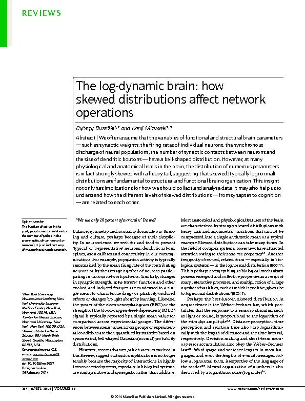
Neuroscience 0 2 4 6 0 200 400 0 100 200 300 10 1 01 001 Firing rate Hz Firing rate Hz Number of cells Mean in linear scale Median Mean in log scale 10

Presentation Embed Code

<iframe width="560" height="315" src="https://www.docslides.com/embed/430206" frameborder="0" allowfullscreen></iframe>

Download Presentation

Download Presentation The PPT/PDF document "Nature Reviews" is the property of its rightful owner. Permission is granted to download and print the materials on this website for personal, non-commercial use only, and to display it on your personal computer provided you do not modify the materials and that you retain all copyright notices contained in the materials. By downloading content from our website, you accept the terms of this agreement.