BIS Quarterly Review, December 2003 Jeffery D Amato+41 61 280 8434jef - PDF document

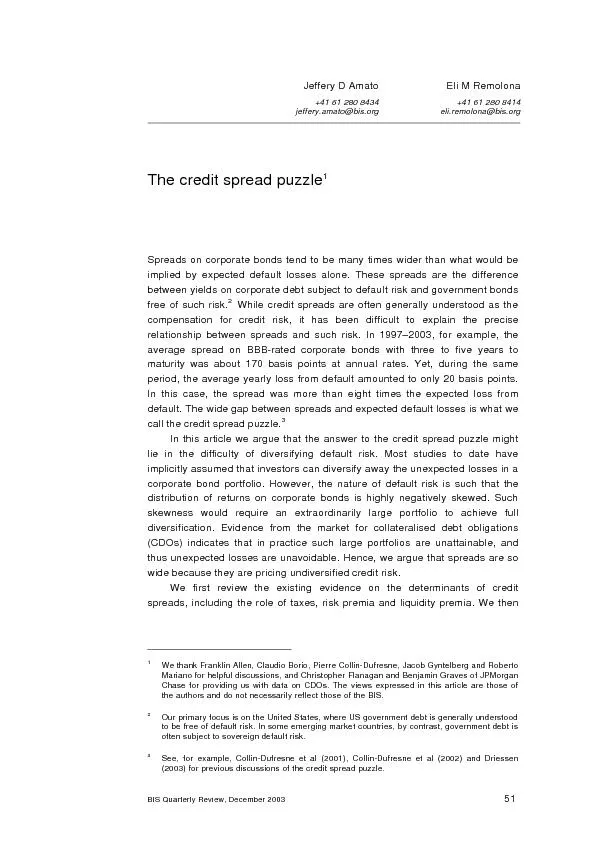
BIS Quarterly Review, December 2003 Jeffery D Amato+41 61 280 8434jeffery.amato@bis.orgEli M Remolona+41 61 280 8414eli.remolona@bis.org Spreads on corporate bonds tend to be many times wider than what would be implied by expected default losses alone. These spreads are the difference between yields on corporate debt subject to default risk and government bonds free of such risk. We thank Franklin Allen, Claudio Borio, Pierre Collin-Dufresne, Jacob Gyntelberg and Roberto Mariano for helpful discussions, and Christopher BIS Quarterly Review, December 2003 discuss the role of unexpected losses and the difficulties involved in diversifying credit portfolios, drawiDecomposing the spreads Average spreads on US corporate debt across rating categories and maturity buckets are given in Table 1. These values are computed using option-adjusted spread (OAS) bond indices provided by Merrill Lynch. The period covered is January 1997 to August 2003. Spreads on AAA debt have averaged about 50 basis points at short maturities and 74 basis points at maturities of seven to 10 years. Spreads increase significantly at lower ratings down to BBB, and even more so across sub-par investment grade debt, reaching as high as 761 basis points on B-rated bonds at one- to three-year maturities. In addition, the term structures are upward-sloping for the higher-rated investment grade bonds, hump-shaped for BBB debt and downward- Maturity 1–3 years 3–5 years 5–7 years 7–10 years Spread Expected Spread Expected Spread Expected Spread Expected AAA 49.50 0.06 63.86 0.18 70.47 0.33 73.95 0.61 58.97 1.24 71.22 1.44 82.36 1.86 88.57 2.70 88.82 1.12 102.91 2.78 110.71 4.71 117.52 7.32 BBB 168.99 12.48 170.89 20.12 185.34 27.17 179.63 34.56 421.20 103.09 364.55 126.74 760.84 426.16 691.81 400.52 In basis points. Spreads are averages over the period January 1997–August 2003 of Merrill Lynch option-adjusted indices for US corporate bonds. See text for details on computation of expected loss. Sources: Altman and Kishore (1998); Bloomberg; Moody’s Investors Service; authors’ calculations. Table 1 See Amato and Remolona (2003) for a more detailed analysis of the issues examined in this The option adjustment is done for callable bonds, for which the premium on the embedded option needs to be taken into account. While it would be desirable to compute averages over longer time periods to ensure that all purely cyclical effects have been cancelled out, OAS corporate bond indices are not available for an earlier period. Spreads computed as the difference between the yield on a corporate bond index and a treasury index of similar maturity, for which longer time series are available, can be misleading (see Duffee (1996)). One potential bias not corrected for in the OAS indices demarcated by rating category is the effect of ratings migration of individual bonds. The rating of each constituent of a particular index at any point in time is required to be the same as the rating of the index. However, this is mainly a problem in assessing changes in yields of a given set of bonds, whereas the focus here is on the level of yields. To economise on notation, we will use only the rating codes of Standard and Poor’s throughout this article. Hence, an “AAA” rating should be taken to mean also the Moody’s “Aaa” rating. Average spreads are high, especially on low-rated bonds BIS Quarterly Review, December 2003 sloping for the sub-par investment grade segment. Moreover, at all maturities, spreads are inversely related to the rating grade, suggesting that ratings are indeed linked to credit quality. As mentioned above, one obvious component of spreads is the expected loss on corporate bonds due to default. Estimates of expected loss are also provided in Table 1, next to the corresponding value of the spread. Expected loss is computed using an (unconditional) one-year ratings transition matrix – indicating probabilities of downgrades as well as defaults – and by assuming that recovery rates are a constant share of face value. The transition matrix is based on historical Moody’s rating changes and defaults, and the estimates of recovery rates are taken from Altman and Kishore (1998). At a given time years into the future, the expected loss is the probability of an issue defaulting within the next years times loss given default. Expected losses are then averaged across the years for each maturity bucket.The most striking feature in Table 1 is that, across all rating categories and maturities, expected loss accounts for only a small fraction of spreads. For BBB-rated bonds with three to five years to maturity, for example, the expected loss amounts to only 20 basis points, while the average spread is 171 basis points. In general, spreads magnify expected losses, but the relationship is not one of simple proportions. For example, while the average spread on BBB-rated bonds with three to five years to maturity is more than eight times the le for AAA-rated bonds is 355 times.Perhaps a more relevant feature of the relationship between spreads and expected losses is that the difference between them increases in absolute terms as the credit rating declines. As shown in Table 1, this difference increases from 64 basis points for AAA-rated bonds with three- to five-year maturities to 291 basis points for B-rated bonds with the same maturities. This absolute difference is important because it gives rise to arbitrage opportunities, The fact that expected loss on US corporate debt appears to be only a small part of the total spread over Treasuries has prompted a search for other factors. Recent work has explored the role of taxes, risk premia and liquidity premia. The remainder of this section briefly discusses each of these in turn. As a benchmark for our discussion, and to illustrate some results in the empirical literature, Table 2 documents the findings of two recent studies using These recovery rates, in percentages, are 68.34 (AAA), 59.59 (AA), 60.63 (A), 49.42 (BBB), 39.05 (BB), 37.54 (B) and 38.02 (CCC). One potential critique of our calculation of expected loss is that it is based on constant recovery in the event of default and unconditional transition matrices constructed using data over a long time period. Instead, we could have computed expected losses by allowing these to vary over time. See, for example, Nickell et al (2000) for a discussion of time-varying transition matrices; Frye (2003) on the relation between probabilities of default and recovery rates; and Altman et al (2003) for an analysis of the link between default and recovery rates. In the language of modern finance, the “risk neutral” probabilities for BBB-rated bonds are eight times the “physical” probabilities. Investors are compensated for expected loss ... … but spreads are many times wider than loss estimates Other factors drive spreads BIS Quarterly Review, December 2003 Spread component Attributed portion of spread (in percentages) Rating AA A BBB Maturity 5 10 5 10 5 10 Elton et al (2001) Expected loss 3.5 8.0 11.4 17.8 20.9 34.7 Taxes 72.6 58.0 48.0 44.1 29.0 28.4 Risk premium 19.4 27.6 33.0 30.9 40.7 30.0 4.5 6.4 7.7 7.2 9.4 7.0 Driessen (2003) Taxes 57.1 55.0 50.8 48.5 37.4 34.0 Risk premium 17.9 23.3 26.2 32.4 45.8 52.1 Liquidity premium 25.0 21.7 23.0 19.1 16.9 13.8 Approximation based on authors’ calculations. Sources: Driessen (2003); Elton et al (2001). Table 2 US data. Elton et al (2001) decomposed spot rates on corporate bonds into expected loss, taxes and a residual. They then examined how much of the variation over time in the residual sp systematic risk factors, and calculated a risk premium based on these contributions. The more recent paper by Driessen (2003) employs different methods and data to further decompose spreads, in particular by allowing for a liquidity premium.In the United States, corporate bonds are subject to taxes at the state level, whereas Treasury securities are not. Since investors compare returns across instruments on an after-tax basis, arbitrage arguments imply that the yield on corporate debt will be higher to compensate for the payment of taxes. Maximum marginal tax rates on corporate bonds vary roughly from 5 to 10% across states. Taking account of the deduction of state taxes from federal tax, Elton et al (2001) use a benchmark tax rate of 4.875% to find that taxes can account for 28–73% of spreads depending upon rating and maturity (see Table 2). Using a different sample and methods, Driessen (2003) finds that Clearly, there are many other studies that we do not discuss here. Our apologies to other authors. We stress that Table 2 and the discussion in the text are meant to be indicative rather than exhaustive. See Amato and Remolona (2003) for a more complete review of the literature. More specifically, Elton et al (2001) first regress the spread less the expected loss and tax components on the three Fama-French (1993) risk factors (market, SMB, HML). The risk premium is then determined by summing across factors the sensitivity of the residual spread to each factor multiplied by the price of each factor. More precisely, Driessen (2003) decomposes spreads into the following categories: taxes, liquidity risk, common factors risk, default event risk, default-free factors risk and firm-specific factors risk. To simplify our presentation, we have combined the last four categories under the heading risk premium. After-tax returns matter BIS Quarterly Review, December 2003 taxes may account for 34–57% of spreads. Since such taxes are more closely related to the level of yields than to the spread, their effect is roughly constant across rating classes, and thus they explain a smaller fraction of the spread on lower-rated bonds than on higher-rated bonds. Risk premium The fact that the unexplained spread is itself volatile adds to the risk of corporate bonds. Moreover, this additional risk cannot easily be diversified away by holding stocks in the same portfolio. Hence, risk-averse investors would require a premium for bearing this risk, in addition to compensation for expected (ie average future) losses and taxes. Elton et al (2001) suggested that such a risk premium might account for anywhere between 19 and 41% of spreads (see Table 2). Driessen (2003) estimated risk premia in a fully specified model and found that they account for a fraction of spreads as low as 18% (AA, five-year maturity) and as high as 52% (BBB, 10-year maturity). Note that such risk premia help suggest why the unexplained spread is so wide, not why it exists at all.Liquidity premium Even in the United States, most corporate bonds trade in relatively thin markets. This means that it is typically more costly to undertake transactions in these instruments than in equities and Treasuries. Investors must be compensated for this. For example, Schultz (2001) estimates that round-trip trading costs in the US corporate bond market are about 27 basis points. More generally, there can be uncertainty about the liquidity (or illiquidity) of a given bond at a given time, and investors might also require a premium to bear this Indeed, several recent studies have argued that liquidity premia may be the next most important component of spreads after taxes. Driessen (2003) estimates that liquidity premia account for about 20%, with Perraudin and The difficulty of diversification A neglected explanation for the size of credit spreads is the difficulty of diversifying credit risk. In corporate bond portfolios, there is often a chance that actual losses from default will exceed expected losses. All the studies Collin-Dufresne et al (2001) find that changes in the spread tend to be highly correlated across issuers but are unrelated to macroeconomic and financial variables. A related but conceptually distinct issue is liquidation risk (see Duffie and Ziegler (2003)). Even for buy and hold investors there is always a chance that positions will have to be liquidated under tight market conditions. Thus, investors will require a premium to bear this risk. However, since the probability of such events is very small, it seems implausible that liquidation risk could induce a large premium. See also, for example, Delianedis and Geske (2001), Dignan (2003), Janosi et al (2001) and Longstaff et al (2003). Returns are risky … … and the market is not so liquid BIS Quarterly Review, December 2003 Medium portfolio Large portfolio -75-60-45-30-150 -40-35-30-25-20-15-10-50 Probabilities on the vertical axis and portfolio losses in thousands of US dollars on the horizontal axis. Probabilities are computed using the binomial distribution. Holding 100 bonds with $30,000 face value each. Holding 300 bonds with $10,000 face value each. Source: BIS calculations. Graph 1 mentioned above implicitly assume that investors can diversify away this unexpected component of default risk by holding a sufficiently large portfolio. This assumption, however, may not hold in practice. Without full diversification, unexpected losses will be priced in the spread. Indeed, we argue that this risk could very well account for most of the spread. Skewness in returns is a critical factor that stands in the way of diversification. Because of this factor, corporate bond portfolios are not as easy to diversify as equity portfolios. Default risk for corporate bonds means there is a small but significant probability of a large loss without any chance for a comparably large gain. The resulting distribution of returns is negatively skewed, that is, it has a long left tail. Given such skewness, diversification is difficult in the sense that the size of the portfolio required to reduce unexpected losses to a minimum is very large. We argue that in practice such large portfolios are not attainable. In contrast, equity returns tend to show a much more symmetric distribution, in which the probabilities of large losses are matched by the probabilities of large gains. Such symmetry makes diversification relatively easy for equity portfolios, and a portfolio with as few as 30 stocks could be considered well diversified. This is not so for a portfolio with To illustrate the difficulty of diversifying credit risk, consider two hypothetical corporate bond portfolios worth a total of $3 million each and divided equally among 100 and 300 different obligor names, respectively.Assume further that these names have identical default probabilities and To keep things simple, we account only for the probability of default. In practice, losses can also arise from downgrades and wider spreads, which would presumably increase the correlation of losses in portfolios. In general, it is important to account for this by integrating credit and market risk. Duffie and Singleton (2003), for example, show how this might be Skewness is the BIS Quarterly Review, December 2003 independent default times. Graph 1 shows the probabilities of varying amounts of default losses for these portfolios, where the default probability of each obligor is 0.5% and the recovery rate in the event of default is 50%. The binomial density is used to compute the probabilities. For both portfolios, the expected loss is $7,500. However, the probabilities of much greater losses than this are significant in both cases. For example, in the medium-sized portfolio with 100 names, there is a greater than 1% probability that losses would be as large as $45,000, six times the expected loss. Note that such unexpected losses are already in the order of magnitude of the credit spreads. Diversification is improved by increasing the size of the portfolio from 100 to 300 names, but it still remains poor: a loss of $25,000 can occur with a probability exceeding 1%, a loss that is more than three times the expected loss. Evidence from arbitrage CDOs Can investors actually hold corporate bond portfolios that are large enough to be fully diversified? One way to address this question is to examine CDOs, particularly arbitrage CDOs. These are vehicles for securitisation that rely on lower-rated debt securities as collateral and issue several tranches of notes, the bulk of which are typically AAA-rated securities. Arbitrage CDOs are particularly interesting for our purposes because they are structured precisely to exploit credit spreads that are wide relative to expected losses, and their success depends on how well they can diversify default risk. The extent to evidence of what is attainable. The basic logic of arbitrage CDOs is simple: take a long position in low-quality debt paying high spreads and take a short position in high-quality debt paying low spreads. Ordinarily, this would be a risky strategy, because it would lose money if spreads widened (spreads would widen more on the long position than on the short position). What makes the strategy an arbitrage, however, is that CDOs take the risk of widening spreads out of the equation by effectively transforming the low-quality debt into high-quality debt at the outset without giving up much of the spread differential. The transformation involves treating the low-quality debt as collateral and setting aside part of it to cover possible losses from default. This strategy works because the gap in spreads between the two classes of debt is much wider than the gap in expected default losses. To illustrate the strategy, consider a collateral pool of BBB-rated bonds, each of which has an independent default probability of 0.5% a year and a recovery rate of 50%, as in the above hypothetical examples. In this case, the expected loss will amount to 25 basis points in annual terms. Suppose the credit spread paid on these bonds is 175 basis points. If the collateral pool is large enough to be perfectly diversified, the CDO manager will not need to be concerned about unexpected losses from default. If 0.25% of the collateral pool is set aside to cover expected losses, the remaining collateral will constitute a We discuss the role of correlations below. Actual losses could be a multiple of expected losses CDOs exploit the credit spread … gaining from the spread differential BIS Quarterly Review, December 2003 portfolio that has no default risk. The manager can then issue AAA-rated bonds against this essentially risk-free portfolio. The gain from this arbitrage strategy will be the spread differential between BBB-rated and AAA-rated bonds minus the cost of overcollateralisation. If the spread on AAA-rated bonds is 50 basis points, this gain will be 100 basis points (125 basis points for the spread differential and 25 basis points for overcollateralisation), an extraordinarily large arbitrage gain. In practice, however, the arbitrage opportunities available are not so attractive, because CDO managers seem unable to assemble perfectly diversified collateral pools and therefore need to set aside much larger amounts of collateral to cover unexpected losses from default. To provide an example, Graph 2 shows the structure of a typical CDO, the Diamond Investment Grade CDO. The collateral is a mix of different types but is mainly composed of BBB bonds. The total number of issuers represented in the collateral pool is 136. However, the “diversity score” assigned by Moody’s suggests that the possibility of default correlations would make the effective number of independent obligors closer to 60 (the role of correlations will be discussed further below). It can be inferred on the basis of Graph 1 that the distribution of potential losses for a portfolio of 60 independent obligors assigns a significant probability to large unexpected losses, and the portfolio is therefore not well diversified. The CDO issued notes in four tranches, with the senior AAA tranche amounting to 83% of the total face value. The equity portion of 4% plus the other tranches of 13% represent the overcollateralisation required to protect the AAA tranche from losses from defaults in the collateral Collateral types Collateral ratings Number of assets 6090 Cash Synthetic Bonds AaaBa1 70105 Issuers Diversity 6090 A3 class B1 Equity In percentages. Structured finance securities. Source: JPMorgan Chase. Graph 2 In evaluating CDOs, Moody’s assigns a diversity score to the pool of collateral. The diversity score is intended to measure the size of the collateral pool in terms of the equivalent number of obligors with independent default times. Thus, the scores reflect default correlations as estimated by the rating agency. The impact of correlation on diversification is discussed below. … and need to be covered by lower tranches But unexpected large … BIS Quarterly Review, December 2003 Diversification and overcollateralisation in CDOs The amount of overcollateralisation is effectively determined by rating agencies: they calculate the amount that will be sufficient to protect the higher-rated tranches against defaults in the collateral pool at probabilities consistent with the ratings of those tranches. The amount of protection will depend largely on the likelihood of unexpected losses in the collateral pool, and these losses will depend on how well diversified the pool is. The relationship between overcollateralisation and diversification can be discerned from the graph below. The three curves in the left-hand panel correspond to collateral pools of different sizes. The graph plots the probability that the proportion of defaults in the collateral pool will exceed the overcollateralisation ratio, which is shown on the horizontal axis. The graph shows that the bigger the collateral pool, the smaller the probability that the proportion of losses will exceed a given overcollateralisation ratio. The required ratio is then set so that this probability is consistent with the default probability associated with a AAA rating, which is the rating of the tranche being protected by the collateral. As shown in the middle panel, the required overcollateralisation ratio is the intersection between the curve for loss probabilities and the horizontal line representing the default probability for the senior tranche. This ratio is smaller for the larger collateral pool. In other words, diversification reduces the proportion of collateral required to cover unexpected losses at a given level of confidence. The right-hand panel shows the arbitrage gains relative to the size of the pool. In this example, the gains roughly amount to the spread differential between BBB and AAA bonds multiplied by the difference in asset size between the senior and equity tranches. The fact that the overcollateralisation ratio continues to decline with the size of the collateral pool means that arbitrage gains also increase. Benefits of diversification Loss probabilitiesRequired overcollateralisation 0.20.40.60.020.030.040.050.06 0.0050.010.0150.080.090.100.110.12 Large portfolio Medium portfolio Small portfolio AAA² 150 Ratio with fulldiversification Required ratio The horizontal axis is the ratio of the number of assets in default () to the total number of assets (). The vertical axis is the probability that the proportion of defaults is greater than Probability of default of a AAA-rated bond over a five-to seven-year horizon. The horizontal axis plots the total number of bonds in the collateral pool (). The minimum collateralisation ratio () is the minimum size of the equity tranche (in percentages) required to achieve a AAA rating for the senior tranche of a two-tranche CDO. The calculations assume that the collateral pool consists of BBB-rated bonds with identical probabilities of default ( = 0.03) over a five- to seven-year horizon and independent default times. The ratio with full diversification is equal to pB–pA, where = 0.001 is the probability of default of a AAA-rated bond over a five- to seven-year horizon. Source: BIS calculations. pool. Since the expected loss is small, most of the required overcollateralisation represents coverage for unexpected losses. For CDO managers, the required overcollateralisation represents a cost that reduces the gains from arbitrage. Such overcollateralisation in turn depends on the degree of diversification achieved in the collateral pool. The BIS Quarterly Review, December 2003 For CDOs based on cash collateral and cash flow management Investment grade High-yield Total 521.1 391.6 Tranches Senior Mezzanine Equity Number of assets3 100 150 Diversity score Averages, at issuance, over the period January 1997–August 2003. In millions of US dollars. Approximate. Source: JPMorgan Chase. Table 3 more diversified the pool, the less the collateral needed to cover unexpected losses from default and the greater the arbitrage gain (see box on page 59 for an illustration). Hence, the benefits of diversification provide the CDO manager with a strong incentive to increase the size of the collateral pool or, more specifically, the number of independent names in the pool. It is significant that in spite of the strong incentive to diversify, actual arbitrage CDOs do not become very large. The typical arbitrage CDO structured on investment grade assets contains only about 100 names in its collateral pool, resulting in an average diversity score of only about 40 (Table 3). Only a few CDOs have had more than 200 names. Conversations with market participants suggest that it can take many months for a CDO manager to assemble the collateral for a given structure. It appears that beyond a few benchmark bonds, the cost of searching for additional names rises sharply. Indeed, the fact that the most common collateral tends to be investment grade debt rather than high-yield debt, for which potential arbitrage gains should be larger, suggests that the availability of collateral is an important limiting factor. Hence, full diversification is not achieved even by investors who would have the most to gain. The practical difficulties of diversification imply that investors cannot fully avoid the risk of unexpected losses from default. In actual portfolios, such risk remains significant and must therefore command a risk premium. It is this risk premium that we believe accounts for much of the credit spread puzzle. The role of default correlations To the extent that defaults tend to occur at the same time, the scope for diversification is more limited. In the extreme, a portfolio with, say, 100 names but with 100% default correlation would have the risk profile of a portfolio with a single name. In practice, default correlations have been difficult to estimate Other factors, such as moral hazard, might also limit profit opportunities. See Duffie and Singleton (2003) and Amato and Remolona (2003) for further discussion. Yet CDO managers do not fully diversify … … so wide spreads reflect undiversified BIS Quarterly Review, December 2003 with any precision. Nonetheless, there are two main factors that are understood to determine default correlations between two firms, their credit quality and whether they are in the same industry. First, the higher the probabilities of default, the more likely that two firms will default together. Zhou (1997) and Gersbach and Lipponer (2003), for example, analytically derive default correlations from asset correlations, the latter serving as an upper bound on the former. Zhou explains that for two firms of low credit quality and a given asset correlation, it will not take much of a decline in asset values for the default of one to be followed by the default of the other. Gersbach and Lipponer provide a numerical example in which an asset correlation of 40% and a default probability of 1% lead to a default correlation of 8%, while the same asset correlation but a default probability of 5% lead to a default correlation of 14%. Second, two firms in the same industry are more likely to default together than two firms in different industries. After all, the business risks faced by firms within the same industry are likely to be similar and asset correlations are likely to be high. Indeed, market participants often assume that default correlations are significantly positive for firms in the same industry and negligible for firms in different industries. Intra-industry estimates from Moody’s based on a large sample of speculative grade firms range from a correlation of 6% for banking firms to 1% for technology firms. Das et al (2001) derive estimates that are as high as 25% for firms in the same industry. However, in general, such correlation estimates tend to be low. While default correlations limit the scope for diversification, they are not what makes corporate bond portfolios so difficult to diversify by comparison with other assets. The fact that equity returns are much more highly correlated than default probabilities means there is less that is diversifiable in equity portfolios. Given what is diversifiable, however, it is harder to achieve full diversification in corporate bond portfolios because of the skewness in returns. As mentioned above, a small equity portfolio can be well diversified in that the idiosyncratic risk of individual stock returns is negligible, while a large corporate bond portfolio is likely to remain poorly diversified in that unexpected losses from default remain significant. Conclusions and implications In this article we have examined various possible sources for the spreads observed on US corporate bonds relative to US Treasuries. We provided calculations confirming the stylised fact that expected losses in the event of default can account for only a small portion of observed spreads. We then There is a large theoretical literature on estimating default correlations. Popular approaches include “copula” and “intensity” models, which tend to rely on parameters derived from estimates of the “lower tail dependence” between asset values of borrowing firms. See Duffie and Singleton (2003). High correlations lead to time variation in default rates. For example, an average probability of default of 1% in a portfolio of 1,000 bonds could mean 10 defaults a year in the absence of a correlation or 20 defaults every other year in the presence of correlation. Lower credit ratings mean higher correlations Correlations across industries are small Correlations are less important than BIS Quarterly Review, December 2003 reviewed arguments and evidence regarding the importance of other factors. While taxes, risk premia and illiquidity may contribute to spreads, they still do not fully explain why spreads are so wide. We suggest instead that the spreads are largely a compensation for the risk of unexpected losses from default that are invariably present in corporate bond portfolios. Unexpected losses are difficult to avoid because default risk leads to returns that are highly negatively skewed. Given this skewness, unexpected losses can be diversified away only with extraordinarily large portfolios. We suggest that such large portfolios are not attainable in practice. For evidence, we turn to arbitrage CDOs, the managers of which have a strong incentive to diversify. The relatively small number of bonds included in actual arbitrage CDOs lends support to the view that diversification is difficult. Beyond a limited number of benchmark bonds, the cost of finding additional bonds seems to rise Apart from the implications the supply of corporate bonds has for diversification, there are other technical issues specific to credit markets that we have largely ignored. The development of derivatives markets, and the fact that certain market participants have taken large gambles involving different credit instruments such as CDOs and CDSs, has surely had an impact on spreads at times. How important these factors are for the average level of spreads remains an open question. Our arguments regarding the difficulty of diversifying credit risk and the subtleties involved in identifying liquidity premia call for more work on both of these issues. Moreover, the ongoing development of credit derivatives has the possibility to transform credit markets even more in the future, particularly with regard to diversification opportunities and market liquidity. This is likely to reduce spreads over the long run, but the size and pace of these effects is yet to be determined. In the end, a better understanding of corporate bond spreads will help improve risk management of defaultable securities and the liquidity of portfolios. It should also lead to improvements in pricing, and hence efficiency, in the markets for corporate bonds and credit derivatives. References Altman, E I and V M Kishore (1998): Defaults and returns on high yield bonds: analysis through 1997Altman, E I, B Brady, A Resti and A Sironi (2003): “The link between default and recovery rates: theory, empirical evidence and implications”, Journal of Amato, J D and E Remolona (2003): Is there a credit premium puzzle?, mimeo, BIS. Collin-Dufresne, P, R Goldstein and J Helwege (2002): Is credit event risk priced? Modeling contagion via the updating of beliefs, mimeo, Carnegie Diversified portfolios are unattainable … … because not enough bonds can be found BIS Quarterly Review, December 2003 Collin-Dufresne, P, R Goldstein and J Spencer Martin (2001): “The determinants of credit spread changes”, Journal of Finance, vol LVI, no 6, December, pp 2177–207. Das, S R, G Fong and G Geng (2001): “Impact of correlated default risk on Journal of Fixed Income, December, pp 9–19. Delianedis, G and R Geske (2001): “The components of corporate credit spreads: default, recovery, tax, jumps, liquidity and market factors”, , the Anderson School at UCLA. Dignan, J H (2003): “Nondefault components of investment-grade bond spreads”, Financial Analysts JournalDriessen, J (2003): Is default event risk priced in corporate bonds?, mimeo, University of Amsterdam. Duffee, G R (1996): Treasury yields and corporate bond yield spreads: an empirical analysisDuffie, D and K J Singleton (2003): Credit risk: pricing measurement and management, Princeton University Press. Duffie, D and A Ziegler (2003): “Liquidation risk”, Financial Analysts JournalElton, E J, M J Gruber, D Agrawal and C Mann (2001): “Explaining the rate spread on corporate bonds”, Journal of Finance, vol LVI, no 1, February, Fama, E and K French (1993): “Common risk factors in the returns on stocks Journal of Financial EconomicsFrye, J (2003): “A false sense of security”, Gersbach, H and A Lipponer (2003): “Firm defaults and the correlation effect”, European Financial Management, vol 9, pp 361–77. Janosi, T, R Jarrow and Y Yildirim (2001): Estimating expected losses and liquidity discounts implicit in debt prices, mimeo, Cornell University, Ithaca. Longstaff, F, S Mithal and E Neis (2003): The credit default swap market: is credit protection priced correctly?Nickell, P, W Perraudin and S Varotto (2000): “Stability of rating transitions”, , 24, pp 203–27. Perraudin, W R M and A P Taylor (2003): Liquidity and bond market spreadsmimeo, Bank of England. Schultz, P (2001): “Corporate bond trading costs: a peek behind the curtain”, , vol LVI, no 2, April, pp 677–98. Zhou, C (1997): “Default correlation: an analytical result”, FEDS paper 1997–27, Federal Reserve Board, May.