/
The Laplace Transform The Laplace Transform

The Laplace Transform - PowerPoint Presentation

olivia-moreira
olivia-moreira . @olivia-moreira
Follow
616 views
Uploaded On 2016-07-30

The Laplace Transform - PPT Presentation

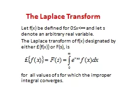
Let fx be defined for 0xlt and let s denote an arbitrary real variable The Laplace transform of fx designated by either fx or Fs is for all values of s for which the improper integral converges ID: 425267

transforms laplace inverse transform laplace transforms transform inverse functions property properties variable constant integral solve appendix improper form equations number elementary differential

Share:

Link:

Embed:

Download Presentation from below link

Download Presentation The PPT/PDF document "The Laplace Transform" is the property of its rightful owner. Permission is granted to download and print the materials on this web site for personal, non-commercial use only, and to display it on your personal computer provided you do not modify the materials and that you retain all copyright notices contained in the materials. By downloading content from our website, you accept the terms of this agreement.


Presentation Transcript

Slide1

The Laplace Transform

Let f(x) be defined for 0≤x<∞ and let s denote an arbitrary real variable. The Laplace transform of f(x) designated by either £{f(x)} or F(s), isfor all values of s for which the improper integral converges.Slide2

Convergence occurs when the limit

exists. If the limit does not exist, the improper integral diverges and f(x) has no Laplace transform.Slide3

When evaluating the integral in

The variable s is treated as a constant because the integration is with respect to x.Slide4

EXAMPLE

Determine whether the improper integral converges.Slide5

EXAMPLE

Determine whether the improper integral converges.Slide6

EXAMPLE

Determine those values of s for which the improper integral converges.Slide7

Laplace Transforms for a Number of Elementary Functions

Find the Laplace Transform of f(x)=1Slide8

Laplace Transforms for a Number of Elementary Functions

Find the Laplace Transform of f(x)=x2Slide9

Laplace Transforms for a Number of Elementary Functions

Find £{eax}Slide10

Laplace Transforms for a Number of Elementary Functions

Additional transforms are given in Appendix A.Slide11

Properties of Laplace Transforms

Property 1. Ifthen for any two constants C1 and C2Slide12

Properties of Laplace Transforms

Property 2. Ifthen for any constant aSlide13

Properties of Laplace Transforms

Property 3. If then for any positive integer nSlide14

Properties of Laplace Transforms

Property 4. Ifthen if exists, thenSlide15

Properties of Laplace Transforms

Property 5. Ifthen Slide16

Properties of Laplace Transforms

Property 6. If f(x) is periodic with period w, that is , f(x+w)=f(x), then Slide17

Functions of Other Independent Variables

For consistency only, the definition of the Laplace transform and its properties, the above equations are presented for functions of x. They are equally applicable for functions of any independent variable and are generated by replacing the variable x in the above equations by any variable of interest. In particular, the Laplace Transform of a function of t is Slide18

Inverse Laplace Transforms

An inverse Laplace transform of F(s), designated by £-1{F(s)} is another function f(x) having the property that £ {f(x)} =F(s). This presumes that the independent variable of interest is x. If the independent variable of interest is t instead, then an inverse Laplace transform of F(s) is f(t) where £ {f(t)} =F(s). Slide19

The simplest technique for identifying inverse Laplace transforms is torecognize them, either from memory or from a table such as Appendix A. If F(s) is not a recognize form, then occasionally it can be transformed into such a form by algebraicmanipulation. Observe from Appendix A that almost all Laplace transforms are quotients. The recommended procedure is to first convert the denominator to a form that appears in Appendix A and then the numerator.

Inverse Laplace TransformsSlide20

Manipulating Denominators: The method of completing the square converts a quadratic polynomial into the sum of squares, a form that appears in many of the denominators in Appendix A. In particular, for the quadratic

as2+bs+c, where a,b,and c denote constants. Inverse Laplace TransformsSlide21

The method of partial fractions transforms a function of the form a(s)/b(s), where both a(s) and b(s) are polynomials in s, into the sum of other fractions such that the denominator of each new fraction is either a first degree or a quadratic polynomial raised to some power. The method requires only

The degree of a(s) be less than the degree of b(s) and2. b(s) be factored into the product of distinct linear and quadratic polynomials raised to various powers.Slide22

The method is carried out as follows.Slide23

Manipulating Numerators:

A factor s-a in the numerator may be written in terms of the factor s-b, where both a and b are constants, through the identity s-a=(s-b)+(b-a). The multiplicative constant a in the numerator may be written explicitly in terms of the multiplicative constant b through the identity a=(a/b)(b)Slide24

Both identities generate recognizable inverse Laplace transforms when they are combined with:

If the inverse Laplace transforms of two functions F(s) and G(s) exist, then for any constants C1 and C2.Slide25

Denote £{y(x)} by Y(s). Then under very broad conditions, the Laplace transform of the nth-derivative (n=1,2,3,…) of y(x) is

Solutions of Linear Differential Equations with Constant Coefficients by Laplace TransformsSlide26

If the initial conditions on y(x) at x=0 are given by

y(0)=C0 , y’(0)=C1 ,……….. y(n-1)(0)=Cn-1 , then For the special cases of n=1 and n=2Slide27

Laplace transforms are used to solve initial-value problems given by the nth-order linear differential equation with constant coefficients

Together with the initial conditions specified y(0)=C0 , y’(0)=C1 ,……….. y(n-1)(0)=Cn-1Solutions of Differential EquationsSlide28

First, take the Laplace transform of both sides of the differential equation

Thereby obtaining an algebraic equation for Y(s). Then solve for Y(s) algebraically, and finally take inverse Laplace transforms to obtain Slide29

Example

Solve y’-5y=0 ; y(0)=2Solve y’+y=sinx ; y(0)=1Solve y’’+4y=0 ; y(0)=2, y’(0)=2Solve y’’-3y’+4y=0 ; y(0)=1, y’(0)=5