/
Income & Expenditure Income & Expenditure

Income & Expenditure - PowerPoint Presentation

pasty-toler
pasty-toler . @pasty-toler
Follow
444 views
Uploaded On 2017-04-12

Income & Expenditure - PPT Presentation

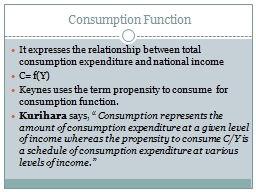
What is the nature of the multiplier and the meaning of aggregate consumption function How do both lead to changes in consumer spending How does expected future income and aggregate wealth affect consumer spending ID: 536763

investment spending consumer income spending investment income consumer disposable current aggregate amp real consumption multiplier gdp function future expected

Share:

Link:

Embed:

Download Presentation from below link

Download Presentation The PPT/PDF document "Income & Expenditure" is the property of its rightful owner. Permission is granted to download and print the materials on this web site for personal, non-commercial use only, and to display it on your personal computer provided you do not modify the materials and that you retain all copyright notices contained in the materials. By downloading content from our website, you accept the terms of this agreement.


Presentation Transcript

Slide1

Income & ExpenditureSlide2

What is the nature of the multiplier and the meaning of aggregate consumption function?

How do both lead to changes in consumer spending?

How does expected future income and aggregate wealth affect consumer spending?

Objectives:Slide3

Producers are willing to supply

additonal

output at a fixed price. As a result, changes in overall spending translate into changes in aggregate outputs as measured by the real GDP

Interest rate as given

No government spending and no taxesExports and imports are zero

Four assumptions:Slide4

What happens if there is a change in investment spending?

Example: Home builders decide to spend an extra $100 billion on home construction in the next year

Each dollar spent on home construction translates into a dollar’s worth of income for construction workers, suppliers of building materials, electricians, etc.

The multiplierSlide5
Slide6

The multiplier

How large is the total effect on aggregate output if we sum the effect from all these rounds of spending increases?

Marginal Propensity to Consume (MPC)

The increase in consumer spending when disposable income rises by $1Slide7

M

arginal Propensity

to Save (MPS) is the fraction of an additional dollar of disposable income that is savedMPS = 1 –

MPC

The multiplierSlide8

With the assumption of no taxes and no international trade, each $1 increase in spending raises both real GDP and disposable income by $1

Increase in investment spending = $100 billion

+ Second-round increase in consumer spending = MPC × $100 billion+ Third-round increase in consumer spending = MPC

2

× $100 billion+ Fourth-round increase in consumer spending = MPC3 × $100 billion • • • • • • • • • • • •Total increase in real GDP = (1 + MPC + MPC2 + MPC3 + . . .) × $100 billion

The multiplierSlide9

The $100 billion increase in investment spending sets off a chain reaction in the economy

The net result -- $100 billion increase in investment spending leads to a change in real GDP that is a

multiple of the size of that initial change in spendingHow large is this multiple?

The multiplierSlide10

Rounds of Increases of Real GDP When

MPC

= 0.6The multiplierSlide11

In the end, real GDP rises by $250 billion as a consequence of the initial $100 billion rise in investment spending:

1/(1 − 0.6) × $100 billion = 2.5 × $100 billion = $250 billion

Notice that endless number of rounds of expansion of real GDP, the total rise in real GDP is limited to $250 billion

Why?

The reason is that at each stage some of the rise in disposable income “leaks out” because it is saved, leaving disposable income is saved depends on MPSThe same analysis can be applied to any other change in spendingThe multiplierSlide12

An autonomous change in aggregate spending is an initial change in the desired level of spending by firms, households, or government at a given level of real GDP.

It autonomous, “self-governing” because it

’s the cause, not the result, of the chain reaction

The multiplier is the ratio of the total change in real GDP caused by an autonomous change in aggregate spending to the size of that autonomous change

The multiplierSlide13

The size of the multiplier depends on MPC

If the MPC is high, so is the multiplier

The multiplierSlide14

The

concept of the multiplier was originally devised by economists trying to understand the Great Depression. Most economists believe that the slump from 1929 to 1933 was driven by a collapse in investment spending. But as the economy shrank, consumer spending also fell sharply, multiplying the effect on real GDP.

In 1929, government in the United States was very small by modern standards: taxes were low and major government programs like Social Security and Medicare had not yet come into being. In the modern U.S. economy, taxes are much higher, and so is government spending.

Why does this matter? Because taxes and some government programs act as

automatic stabilizers, reducing the size of the multiplier. The Multiplier and the Great DepressionSlide15

What determines how much consumers spend?

Consumer SpendingSlide16

Most important factor affecting a family’s consumer spending is its current disposable income (income after taxes & government transfers are received)

Current disposable income & Consumer SpendingSlide17

Consumption Function is an equation showing how an individual households consumer spending varies with the household’s current disposable income

C =

individual household consumer spending

y

d = individual household current disposable incomea = constant term – individual household autonomous consumer spendingCurrent disposable income & Consumer SpendingSlide18

Autonomous

consumer

spending is the amount a household would spend if it had no disposable incomeAssume that a is greater than zero due to a household with no disposable income is able to fund some consumptions by borrowing or using its savings

MPC is expressed as a ratio of change in consumer spending to the change in current disposable income

Current disposable income & Consumer SpendingSlide19

Individual household is shown as:

Multiplying both sides by

Δyd:

When

yd goes up by a $1, c goes up by MPC x $1

Current disposable income & Consumer Spending

MPC

=

Δ

c

/

Δy

d

MPC x

Δy

d

=

Δ

cSlide20
Slide21

Current disposable income & Consumer Spending

Deriving the Slope of the Consumption FunctionSlide22
Slide23

Current disposable income & Consumer Spending

For American Households in 2008, best estimate of the average household’s autonomous consumer spending is:

A

= $17,484

MPC = 0.534 (0.53)Implies that MPS – the amount of an additional $1 of disposable income that is saved1-0.53 = 0.47Multiplier is 1/(1-MPC) = 1/MPS1/0.47 = 2.13

c

= $17,484 + 0.534 x

y

dSlide24

Shows a microeconomic relationship between the current disposable income of individual households and their spending on goods and services

Similar relationship called aggregate consumption functionSlide25

Current disposable income & Consumer Spending

Aggregate consumption function is the relationship for the economy as a whole between aggregate current disposable income and aggregate consumer spending

C =

aggreagte

consumer spending (consumer spending)YD = aggreagate current disposable icnome (disposable income)

A =

aggreagte

autonomous spending, the amount of consumer spending when

Yd

equals zero

C

= A + MPC x Y

DSlide26

The aggregate consumption function shifts in response to changes in expected future income and changes in aggregate wealth.

Current disposable income & Consumer SpendingSlide27

Shifts of the aggregate consumption function

Aggregate consumption function shows the relationship between disposable income and consumer spending of the economy as a whole,

other things equal

When things change other than disposable income, the aggregate consumption function shifts

Two reasons for the shift:Changes in expected future disposable incomeChanges in aggregate wealthSlide28

Changes in expected future disposable income

Effect of good news, information that leads consumers to expect higher disposable income in the future

Consumers spend more, leads to an increase in A-aggregate autonomous consumer spending from A1 to A2

Effect is to shift the aggregate consumption function up, from CF1 to CF2Slide29

Current disposable income & Consumer Spending

Effect of bad news, information that leads consumers to expect lower disposable income in the future

Consumers spend less at any given level of current disposable income

YD corresponding to a fall in A from A1 to A2

Effect is to shift the aggregate consumption function down, from CF1 to CF2

Aggregate consumption function, CF1

Aggregate consumption function, CF2Slide30

Milton Friedman,

A Theory of the Consumption Function

suggest that consumer spending ultimately depends mainly on the income people expect to have over the long term rather than on their current income

Current disposable income & Consumer SpendingSlide31

Maria

Mark

Salary

$30,000

$30,000Work History

10 years

In and out of work

Home

Owns

Rents

Savings

$200,000

No savings

Changes in Aggregate Wealth

Who will spend more on consumption?

Expect Maria but wealth itself has an effect on consumer spendingSlide32

Life-cycle hypothesis – consumers plan their spending over their lifetime, not just in response to their current disposable income

As a result, people try to smooth their consumption over their lifetimes – they same some of their current disposable income during their years of peak earnings and during their retirement live off the wealth they accumulated while working

Wealth affects household consumer spending, changes in wealth across the economy can shift the aggregate

comsumption

functionChanges in Aggregate WealthSlide33

Consumer spending is much greater than investment spending, booms and busts in investment spending tend to drive the business cycle

Most recessions are a fall in investment spending

Investment SpendingSlide34

Planned investment spending is the investment spending that firms

intend

to undertake during a given periodThe level of spending businesses actually carry out is sometimes not the same level as was planned

Planned investment spending depends on three principal factors:

Interest rateExpected future level of real GDPCurrent level of production capacityInvestment SpendingSlide35

Clearest effect on particular form of investment spending: spending on residential construction

Why?

Home builders only build houses that they think they can sellHouses are more affordable, and likely to sell, when the interest rate is low

Also affect forms of investment spending

Firms with investment spending projects will go ahead with a project only if they expect a rate of return higher than the cost of the funds they would have to borrow to finance that projectThe interest rate & investment spendingSlide36

A rise in the market interest rate makes any given investment project less profitable

A fall in the interest rate makes some investment projects that were unprofitable at the now lower interest rate

Planned investment spending – spending on investment projects that firms voluntarily decide whether or not to undertake – is negatively related to the interest rate

Higher interest rate leads to a lower level of planned investment spending

The interest rate & investment spendingSlide37

Current level of productive capacity has a negative effect on investment spending

The higher the current capacity, the lower the investment spending

Effects on investment spending:Growth in expected future sales

Size of current production capacity

Expected future Real GDP, Production capacity, & investment spending

Firms most likely undertake high levels of investment spending – when expect sales to grow rapidlySlide38

What’s an indicator of high expected growth in future sales?

High expected growth of real GDP

Results in a higher level of planned investment spending but a lower expected future growth rate of real GDP leads to lower planned investment spending

Expected future Real GDP, Production capacity, & investment spendingSlide39

Firms maintain inventories

A firm that increases its inventories is engaging in a form of investment spending

Inventory investment is the value of change in total inventories held in the economy during a given periodCan actually be negative

Inventories & unplanned investment spendingSlide40

Unplanned inventory investment occurs when actual sales are less than businesses expected, leading to unplanned increases in inventories

Sales in excess of expectations result in negative unplanned inventory investment

Actual investment spending is equal to planned investment spending plus unplanned inventory investment

Relationship investment spending, unplanned inventory investment and actual investment spending is:

I = IUnplanned + Iplanned

Expected future Real GDP, Production capacity, & investment spendingSlide41

Rising inventories typically indicate positive unplanned inventory investment and a slowing economy

Falling inventories typically indicate a negative unplanned inventory investment and a growing economy

Expected future Real GDP, Production capacity, & investment spending